2026-09-26 · 20 min · quantization · inference-optimization · kernels · triton · vllm · open-source · llm · explainer

On 23 September Red Hat AI announced LLM Compressor v0.14.0: "GPTQ just got its biggest speedup since launch. A new Triton kernel makes quantization ~15x faster end to end. Batching layers that share a shape pushes that to ~30x on some MoE workloads. Even the old eager path is 1.5-2x faster."
I cloned vllm-project/llm-compressor at the 0.14.0 tag (commit 6e4b96e, 22 September),
read the release notes, the pull request that did the work
(#3128) and the benchmark notes its
author linked from it, and wrote a small GPTQ of my own to check the maths. The short version:
- The kernel fuses the innermost loop of GPTQ, the column-by-column quantize-and-update inside each 128-column block. Nothing about the algorithm changed.
- "Batching layers" means stacking same-shaped
Linearmodules from the same calibration stage, typically a layer's 128 experts, into one tensor for the solve. It does not calibrate several transformer layers at once, and it is not sequential onloading. - The 15x and the 30x are real measurements on one H100, but on a calibration set of 2,048 random tokens, where the parts the kernel does not touch are nearly free.
- license
- Apache-2.0
- branch
- HEAD
- tests
- 268 files
- source
- 2.3 MB
- commit date
- 2026-09-22
by size of tracked source at this commit, file counts in brackets; docs, data and vendored trees excluded
local clone, 2026-09-26 at 6e4b96e — branch, commit, commitDate, fileCount, hasTests, languages, license, licenseFile, shallow, testFileCount
shallow clone: counts describe the pinned tree, not the history
The problem GPTQ solves
GPTQ (Frantar et al.) quantizes a trained model one linear layer at a time. Take a layer's weights , with output rows and input columns, and the inputs that reach it when calibration tokens run through the model, a matrix. The grid is fixed beforehand: an observer picks a scale per row or per group, and every quantized weight must be a multiple of it. GPTQ then chooses which grid point each weight gets, to preserve the layer's output:
Write the error as . The objective splits over rows, and for one row ,
So the calibration data enters only through , a matrix that is the same for every row. Round-to-nearest (RTN) minimizes each on its own, which is optimal only if is diagonal. Real layer inputs are not: channels are correlated, so the error from rounding one weight can be cancelled by nudging the weights of channels that move with it. Those weights are still full precision, so they can be moved.
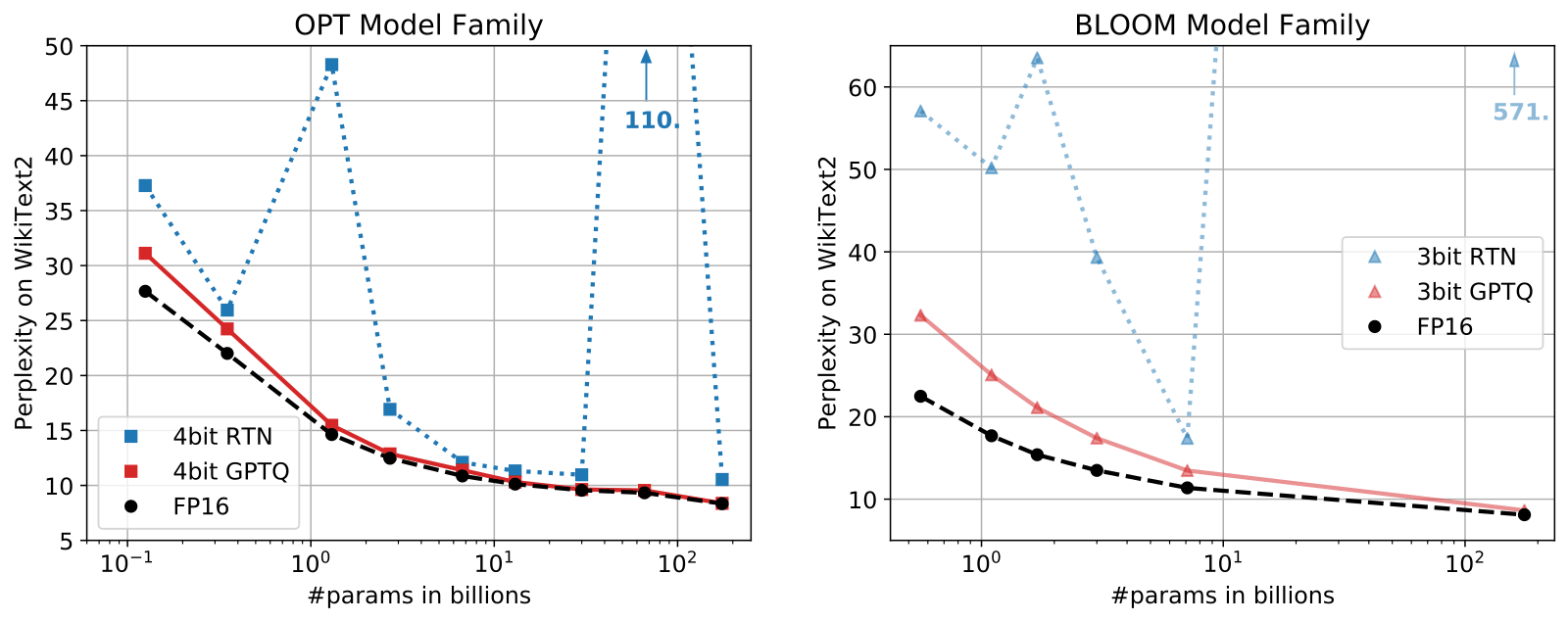
The payoff is not subtle at scale. In the paper's Table 3, plotted in its Figure 1, 4-bit RTN takes OPT-175B from 8.34 WikiText-2 perplexity to 10.54, and GPTQ to 8.37. At 3 bits, RTN takes BLOOM-176B to 571; GPTQ to 8.64.
One weight at a time: the Optimal Brain Surgeon update
GPTQ descends from Optimal Brain Surgeon, a 1993 pruning method, by way of Optimal Brain Quantization (OBQ). Suppose weight of a row is rounded and is the set of weights not yet quantized. The objective is a quadratic with Hessian , and the best compensating change to the weights in has a closed form (the paper's Equation 2):
The error is divided by a diagonal entry of the inverse Hessian and spread along its column. Channels whose inputs track channel get the largest share. Then leaves , and rather than re-inverting, OBQ removes its row and column from with one step of Gaussian elimination:
OBQ picks weights greedily and keeps a separate inverse for every row, which costs . The paper puts it at about an hour for ResNet-50's 25M parameters. A 175B language model is out of reach.
Three changes that make it fast
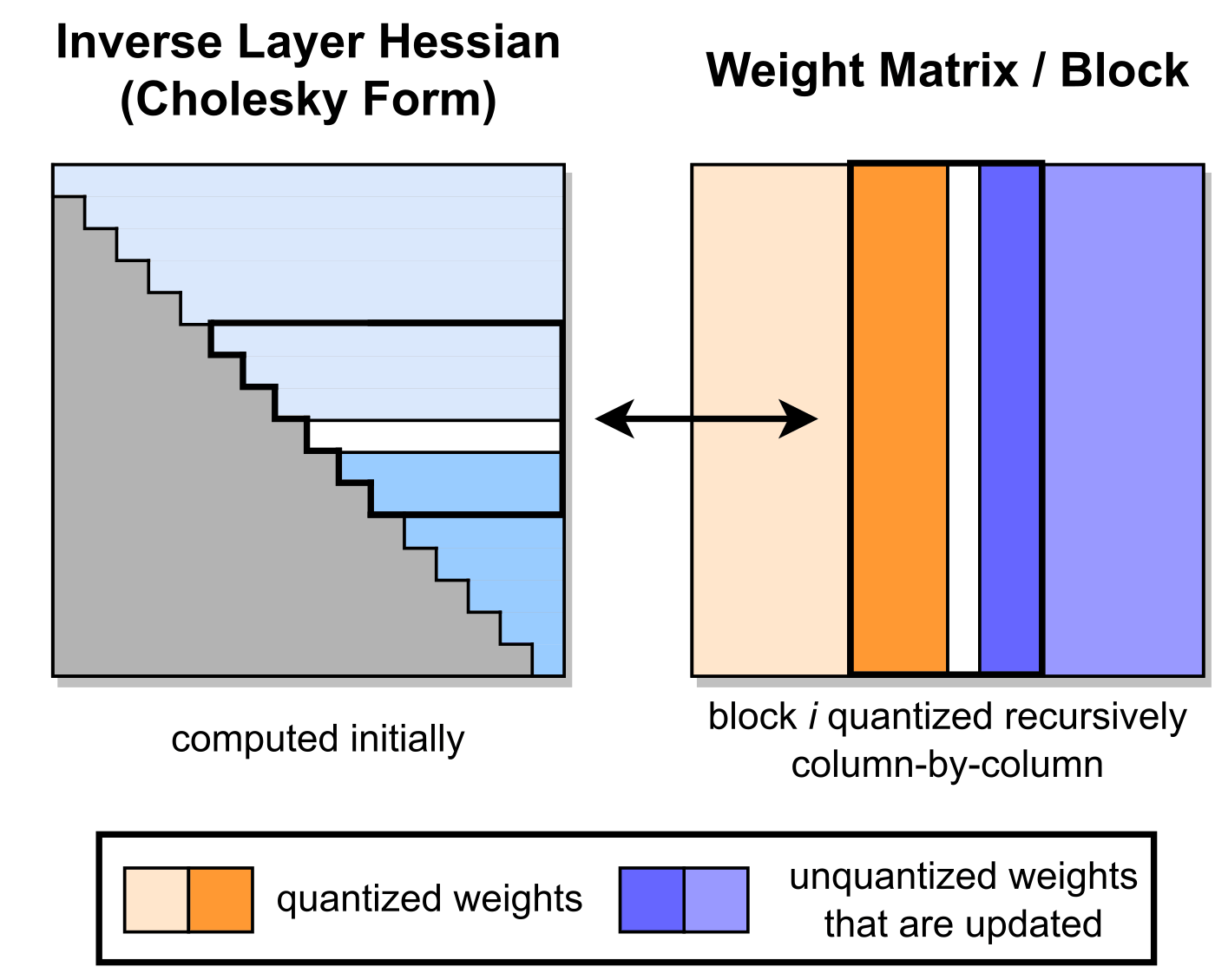
One order for every row. Frantar et al. found that the greedy order buys little on large layers, so GPTQ quantizes columns left to right in every row. Since depends only on , all rows now share one , and the elimination runs once per column instead of once per weight: .
Cholesky instead of repeated elimination. Quantizing column needs only row of the current inverse, from the diagonal onward. Those rows are exactly the rows of the upper Cholesky factor of , up to a scale: . So one factorization up front replaces eliminations, and each column step becomes
Substitute back in and this is the OBS update for all rows at once. The paper adopted it for stability: at scale, accumulated numerical error can leave indefinite, which sends the updates "in incorrect directions".
Lazy blocks. Column 's rounding depends only on updates to column , so the updates to far-away columns can wait. GPTQ works through columns at a time, applies the rank-one updates inside the block, collects the block's errors in a matrix , and only then updates everything to the right with one matrix multiply, . The arithmetic is the same; what changes is that the expensive part becomes a GEMM instead of memory-bound rank-one sweeps.
Dampening. is singular whenever there are fewer calibration tokens than input columns, or a
channel is always zero. GPTQ adds of the mean diagonal to before factorizing.
LLM Compressor does the same (dampening_frac = 0.01), sets dead channels' diagonal to 1 and their
weights to 0, and when the Cholesky still fails, falls back to RTN for that module with a warning.
Here is Algorithm 1 as I wrote it in numpy. It is my code, not the library's:
# gptq_demo.py (mine): Algorithm 1 of arXiv 2210.17323
def gptq(W, H, s, lo, hi, B=128, percdamp=0.01):
    W = W.copy()
    U = inv_chol_upper(H, percdamp)            # dampen, Cholesky, invert, Cholesky (upper)
    Q = np.zeros_like(W)
    for i1 in range(0, W.shape[1], B):
        i2 = min(i1 + B, W.shape[1])
        E = np.zeros((W.shape[0], i2 - i1))
        for j in range(i1, i2):
            Q[:, j] = np.clip(np.round(W[:, j] / s[:, 0]), lo, hi) * s[:, 0]
            e = (W[:, j] - Q[:, j]) / U[j, j]
            E[:, j - i1] = e
            W[:, j:i2] -= np.outer(e, U[j, j:i2])   # inside the block
        W[:, i2:] -= E @ U[i1:i2, i2:]              # lazy update of the rest
    return Q
The widget runs the same loop on a 6 × 12 layer with one block. Step the slider to commit columns and watch the error of each committed column land on the columns to its right; change the input correlation to see when that helps.
- round to nearest
- 0.0256
- GPTQ
- 0.0107
- GPTQ / RTN
- 0.42
- grid points changed
- 13 of 72
Column 3 is on the grid. Its error moved the cells to its right in proportion to the strip above: columns whose inputs track column 3's absorb the most. After all 12 columns GPTQ's output error is 0.42 times rounding's, and it got there by choosing a different grid point for 13 of 72 weights.
Illustrative: the layer and its calibration tokens are seeded random numbers. The update rule, the Cholesky factor and the 1% dampening are GPTQ's, with a single block.
At 3 bits with correlation 0.9, the toy's held-out output error is 0.0107 for GPTQ against 0.0256 for RTN, and GPTQ got there by picking a different grid point for 13 of 72 weights. With uncorrelated inputs, the off-diagonal of the Cholesky factor is only sampling noise from 48 tokens, and GPTQ ends 7% worse than rounding.
The same pattern holds at a more realistic size. On a random 256 × 512 layer, INT4 with a per-row absmax grid, 4,096 calibration tokens, and error measured on 8,192 held-out tokens from the same distribution (all measured, my code):
| Input correlation | RTN error | GPTQ error | GPTQ / RTN |
|---|---|---|---|
| 0 | 0.0185 | 0.0197 | 1.07 |
| 0.5 | 0.0187 | 0.0118 | 0.63 |
| 0.9 | 0.0182 | 0.00305 | 0.17 |
| 0.99 | 0.0190 | 0.00078 | 0.041 |
Three checks from the same script:
- Lazy blocks are exact. Block sizes 1, 8, 128 and 512 give the same quantized matrix: 0 of 131,072 weights differ.
- The Cholesky form is the OBS update. Explicit Equation 2 updates with Gaussian elimination of give the same 131,072 grid points as the Cholesky version.
- Dampening matters when tokens are scarce. With 128 calibration tokens for 512 input columns, has rank 128 and the undamped Cholesky fails. With 1% dampening GPTQ reaches 0.00513 on held-out tokens against RTN's 0.0186; with 0.01% it reaches 0.00789, an overfit to 128 tokens. With 8,192 tokens, dampening anywhere from 0.01% to 10% moves the error by a third of a percent.
Where the wall-clock time goes
LLM Compressor runs GPTQ inside a sequential pipeline: the model is cut into stages, usually one
decoder layer each, and the calibration batches pass through each stage twice. The first pass
fires a hook on every targeted Linear that adds its input to that module's Hessian; the end of the
pass quantizes the stage's modules; the second pass pushes the batches through the now-quantized
stage to produce the next stage's inputs. That is the paper's recipe too: each layer is calibrated
on the outputs of the already-quantized layers before it. The cost has four parts:
| Phase | Where | Scales with |
|---|---|---|
| Two forward passes per stage | pipelines/sequential/pipeline.py | tokens × parameters |
| Hessian accumulation, FP32 per module | accumulate_hessian | tokens × |
| Dampen, Cholesky, invert, Cholesky | factorize_hessian | |
| Column loop, plus one GEMM per block | quantize_weight | FLOPs, sequential steps |
The first two grow with the calibration set; the last two do not. And the last one has a problem that FLOP counts hide. Each column is one sequential step, and in eager PyTorch one step is a string of separate ops: fake-quantize the column (itself several elementwise kernels), subtract, divide, three writes, a square, a multiply and an in-place subtract, each launching a GPU kernel over one column of a few hundred to a few thousand numbers.
The PR's own measurements show what that costs. Llama 3 8B has 32 layers of seven projections; GPTQ walks 32 × (6 × 4,096 + 14,336) = 1,245,184 weight columns. Qwen3-30B-A3B, with 128 experts per layer and every expert calibrated, walks 48 × (3 × 2,048 + 4,096 + 128 × (2,048 + 2,048 + 768)) = 30,375,936. Divide the old code's end-to-end time by those counts (my arithmetic): 214 µs per column on Llama, 219 µs on Qwen. Qwen's expert matrices have 768 or 2,048 rows, Llama's projections 1,024 to 14,336. A cost that does not care how big the column is comes from launching kernels and running Python, not from arithmetic.
What v0.14 changed
The fused kernel
PR #3128, by HDCharles with Isotr0py as co-author, built on an earlier PR (#3109) and merged on
14 September. It routes the per-block loop through a dispatcher in src/llmcompressor/modifiers/gptq/gptq_quantize.py:
gptq_block_update is the eager loop, and _gptq_block_update_triton is registered ahead of it,
taken when the tensors are on CUDA, the scheme is INT, FP4 (E2M1) or FP8 (E4M3), the block width is
a power of two no larger than 256, and LLMCOMPRESSOR_DISABLE_GPTQ_TRITON is not set. The default
block of 128 qualifies.
fused_gptq_block_update launches _gptq_block_update_kernel on a grid of (modules in the batch,
row tiles of 16). Each program loads its 16 × 128 tile of the block on chip and walks the
128 columns itself: divide by the scale, add the zero point, clamp, round, dequantize, compute
, store and , and subtract from the block's columns to
the right. This works because GPTQ's rows are independent once they share the column order. Rows run
in parallel across programs, columns in sequence inside one, and no program ever waits on
another. One launch per block replaces several launches per column.
Details worth knowing:
- Rounding per format. INT rounds with
rint. FP4 rounds through a ladder of thresholds onto , alternating<=and<so that ties go to the even code. FP8 casts tofloat8e4nv; on an A100, which lacks that cast in Triton, it scales by intofloat8e4b15and back, a fix that landed later in #3181. - No fused multiply-adds. Every subtract, multiply and divide in the update goes through the
_rnlibdevice intrinsics, presumably so the compiler cannot contract them into FMAs that the eager path does not use. The tests below demand bitwise equality with the eager loop. - What stays outside. The Cholesky factorization and the block-to-rest update,
torch.bmm(Err1, Hinv[:, i1:i2, i2:]), remain PyTorch calls. They were already dense linear algebra.
Batching "layers"
assign_batches in helpers.py groups the modules that were just calibrated by batch_key: weight
shape, dtype, device and the quantization arguments serialized to JSON. Each group becomes one
[batch, rows, cols] stack of weights and one of Hessians, and quantize_weight runs Cholesky,
kernel and GEMMs over the whole stack. batched_quantization="auto", the default, caps a stack at
75% of free GPU memory, from an estimate of the peak workspace per module. Below 16 modules,
factorize_hessian still factorizes one by one, because the author measured batched CUDA Cholesky
losing at small batch sizes.
Batching happens inside one pipeline stage, on modules calibrated together. A Llama layer yields
three pairs (q/o, k/v, gate/up) and a singleton down_proj. A Qwen3-30B-A3B layer yields a stack
of 256 expert gate_proj and up_proj modules and one of 128 down_proj. What it buys is
fewer, fuller launches. On the Triton path one 768-row expert is 48 programs of 16 rows, fewer than
an H100 has streaming multiprocessors; a stack of 256 is 12,288 programs in one launch. On the eager
path, each per-column op now covers every module in the stack.
The eager path, and one removal
The Python loop got cheaper too. #3097
hoisted a Pydantic copy and two slices out of the per-column loop. #3128 stopped computing
twice, stopped passing an all-zero zero point, and replaced the rank-one update's
[rows × 1] @ [1 × rest] matmul with an elementwise multiply. It also removed
offload_hessians, which on Llama made the PR's own runs seven to eight times slower.
How the 15x and 30x were measured
The PR's benchmark notes give the setup. One H100. W4A16, group size 128. The whole oneshot() call
timed with time.perf_counter(), after the model is loaded and without saving. Two models:
Meta-Llama-3-8B-Instruct resident on the GPU in BF16; and Qwen3-30B-A3B with all 48 layers,
CPU-offloaded and onloaded one stage at a time, with every expert calibrated on every token. Both
calibrated on 8 samples of 256 random token ids.
Dense Llama has only pairs of same-shaped projections, so batching adds almost nothing on the Triton path. The kernel alone takes 266.39 s to 17.90 s.
Measured by the PR author on one H100; ratios are against main without Hessian offload, the default. Per-column figures are my arithmetic.
| Configuration | Llama 3 8B | Qwen3-30B-A3B |
|---|---|---|
| main (pre-PR), Hessian offload | 408.70 s | not completed |
| main (pre-PR), the default | 266.39 s | 6,653.18 s |
| PR eager | 157.61 s | 3,779.61 s |
| PR eager, batched | 115.17 s | 278.94 s |
| PR Triton | 17.90 s | 336.76 s |
| PR Triton, batched | 17.19 s | 212.79 s |
Reported by the PR author. The ratios below are my arithmetic.
The claims check out against their own baseline. Llama: 266.39 s to 17.90 s is 14.9x, or 15.5x with the default batching on. Qwen: 6,653.18 s to 212.79 s is 31.3x. The eager path alone improved 1.69x on Llama and 1.76x on Qwen, inside "1.5-2x". Batching adds 1.58x on Qwen's Triton path and nothing measurable on Llama's.
Two numbers in the table are more interesting than the headline. On the MoE, batched eager GPTQ (278.94 s) beats unbatched Triton (336.76 s): stacking 128 experts amortizes the per-column launch cost just as fusing does. And per column, the PR's eager path costs 127 µs on Llama and 124 µs on Qwen, the same cost on two very different models again. Triton with batching brings it to 14 µs and 7 µs.
What those numbers leave out
The calibration set is tiny. The repo's own Llama 3 example calibrates on 512 samples of up to
2,048 tokens; the benchmark used 8 × 256 = 2,048 tokens, 512 times fewer. The forward passes and
the Hessian accumulation scale with tokens; the column loop does not. So the benchmark isolates
almost exactly the part the kernel speeds up. At the example's size, and with no change in 0.14,
Hessian accumulation alone is FP32 operations: with
it is per Llama layer and for the
model (my arithmetic, an upper bound when samples run short). At an assumed 50 TFLOP/s sustained,
that is about seven minutes, next to a 17.90 s solve. The end-to-end ratio at production settings
will be well below 15x. Nobody measured it. (The ids are torch.randint draws, and 2,048 tokens leave every Llama Hessian, 4,096 or 14,336
columns wide, rank-deficient and invertible only through dampening. Neither changes the timing; both
mean these runs produced no model anyone would evaluate.)
Batching costs memory. On the full Qwen run, peak allocated GPU memory rises from 5.90 GiB unbatched to 15.11 GiB batched. The 75%-of-free-memory rule keeps it inside the card; it does not keep it small.
The harness predates the merged API. It passes batched_quantization as a boolean and a
batch_memory_fraction; the tagged GPTQModifier takes "auto", an integer or None, and
forbids unknown fields. The numbers come from a pre-merge revision of the PR, not the tag.
The docs round up. The release notes say batching reaches "approximately 30× faster end-to-end performance on some MoE workloads", which holds. The docs index adds that batching gives "a further approximately 2x", and the README "up to ~1.67x per batch"; the measured end-to-end gain is 1.58x, and 1.70x is the best single shape in a microbenchmark.
After the kernel, the Cholesky is next. The PR's section timing of one Llama layer puts the fused column updates at 92.8 ms and the block-to-rest GEMMs at 96.1 ms; Hessian factorization, the same code on either path, took 0.369 s in the eager run. Those three add up to 0.56 s a layer, and 32 layers of that is 17.9 s, the measured end-to-end time (my arithmetic). On a dense model the factorization is now two-thirds of the solve.
Is the output the same?
The GPTQ algorithm did not change, so the question is numerical, and the evidence is tests, not evaluations:
- Triton against eager, bitwise.
test_fused_gptq_kernel_matches_eagerassertstorch.equalon the quantized weight, the scales and the loss for a 48 × 64 layer, over INT4 (symmetric and asymmetric, grouped), INT8, FP8 per channel and per block, FP4 grouped and NVFP4, with and without activation ordering. That is fourteen cases, on a layer narrower than one block, so the block-to-rest GEMM is not exercised. - Batched against one at a time, close.
test_quantize_weight_batch_close_to_singleallowsrtol=1e-4andatol=1e-5: a batched GEMM may sum in another order. - Against 0.13, bitwise, then not shown. The benchmark notes record all 224 quantized Llama weights matching the old code bit for bit, but for an "exact parity" revision that kept a separate column-major factor and per-module matmuls. The next revision removed that path for batched linear algebra, and no hash comparison is shown after it. My numpy result above suggests why that is benign: reordering the block arithmetic changed 0 of 131,072 grid choices. At model scale a few weights sitting on a rounding boundary may flip.
- No accuracy numbers. The PR reports none. The repo does carry a nightly
lm-evaluation-harnessgate for GPTQ W4A16 on Llama 3 8B Instruct, GSM8K 5-shot with 512 calibration samples, expecting 0.72 exact match and 94% recovery. Those are thresholds; its results are not in the release.
The observers that "beat GPTQ"
The same release expands the MSE and iMatrix observers, which choose the grid rather than the rounding: they search per-block scales wider than the absmax, a superset of Four Over Six's choice between the absmax and 1.5 times it for NVFP4. The post says they "beat GPTQ for NVFP4 on internal benchmarks". PR #2950 has the table: perplexity deltas on six models, lower is better, averaging +0.139 for the expanded MSE observer, +0.159 for expanded iMatrix and +0.189 for GPTQ. Per model it is closer. GPTQ is lower than expanded MSE on Llama 8B (+0.238 against +0.242), Qwen3-32B (+0.123 against +0.171) and the 30B MoE (+0.096 against +0.149); the average rests mostly on Llama 70B and Qwen3-8B. The table does not say which observer set GPTQ's grid. The two methods compose in principle, since GPTQ rounds onto whatever grid an observer chose. For how NVFP4 is built, see Nemotron in NVFP4.
The takeaway
GPTQ's arithmetic was never the slow part. The algorithm is a sequence of small steps, and in eager PyTorch every step paid launch and interpreter overhead: about 214 µs per column whether the column had 768 numbers or 14,336. The fix is the obvious one once that is visible. Keep a tile of the block in registers, walk the columns inside one kernel, and let the rows run in parallel. For MoE, give the GPU enough rows by stacking experts.
What the speedup buys depends on calibration size. With a production calibration set, the costs that grow with tokens, forward passes and FP32 Hessian accumulation, were always there and are still there. For where quantization sits in serving, see how LLM inference works; for what happens below 4 bits, where the grid itself is the problem, see runtime dynamic compression. And for why a quantization recipe is worth this much care, the Laguna model factory write-up shows naive INT4 costing far more on agentic tasks than on single-turn ones.