μLattice: an open Spotlight-style memory, and what its 7,280x counts

2026-10-13 · 16 min · linear-attention · long-context · attention · kv-cache

Why read this

Recounts μLattice's 7,280x as T/18 (about 114x in multiply-adds), runs its tests on CPU, and shows the bolt-on score equals its closed-answer share.

Checked against the source
Runs on a laptop CPU
Concrete numbers to act on

LLM architectureMITResearch teardown

How this was scored

Is it new?: 1 of 3: An incremental tweak
Can I trust it?: 3 of 3: Reproduces the headline result, or shows from primary files it is wrong
Can I run it?: 2 of 3: Open code or weights with real limits
Will I understand it?: 2 of 3: Mechanism from first principles with figures
Can I act on it?: 2 of 3: A concrete recipe, numbers or comparison
Will it last?: 1 of 3: Relevant for months
Does it affect many?: 1 of 3: A specialist community
Only here?: 2 of 3: A teardown or measurement few others did

Score 63 of 100, ranked 229 of 513 rated articles. Each question is answered 0–3 by hand, and a 3 is rare. How articles are scored

On 12 October Eric E. (@Ex0byt, "Tensorbend Research") posted: "The quadratic memory barrier in AI has been broken. I give you μLattice." The bullet points were memory that grows with the input and has no fixed capacity, orders of magnitude fewer operations than attention, and perfect recall of thousands of associations. The repository (MIT, commit 7af2de3) has a 243-line PAPER.md, a frank LIMITATIONS.md, about 6,000 lines of Python, six checkpoints, result JSONs and a live demo.

This is worth reading closely, and not for the reason the post gives. The mechanism is a real, small, inspectable implementation of an idea I wrote about a week ago in Linear attention's memory problem: Percepta's Spotlight, a memory that grows while each token touches nine cells. Percepta published a blog and no training code. μLattice publishes training code, checkpoints and tests. The source comments say where the design comes from (lattice.py: "Published (Percepta blogs)"; kernel.py: "The BLOG publishes cos^2(pi t / 3)"). PAPER.md itself never says so. It cites Spotlight only as a baseline in one table.

I read the paper, the limitations file, the model, kernel, scan and bolt-on code, and every file in results/. I ran the repository's own unit tests on CPU and tried its acceptance tests there. Every number below is labelled measured (I computed it from a file or a run), reported (the repository's figure, not re-run) or reasoned (my arithmetic on the other two).

Two ways to pay for memory

A sequence mixer has to answer one question at every token: what do I remember about everything before me, and how much do I pay to look it up?

Attention remembers everything. Token $t$ appends a key and a value to the KV cache and scores its query against all $t$ stored keys. Memory grows as $O(T)$ . Compute per token grows as $O(t)$ , so a whole sequence costs $O(T^2)$ comparisons. Recall is exact, because nothing was thrown away. (The memory is linear, not quadratic. FlashAttention never materialises the $T \times T$ score matrix. The quadratic bill is compute.)

A recurrent mixer like Gated DeltaNet keeps one fixed matrix per head. Each token does a constant amount of work on it, so per-token cost is $O(1)$ and a sequence is $O(T)$ . The catch is capacity. A $d_k \times d_v$ state can hold roughly $d_k$ nearly orthogonal key/value associations before they interfere. At μLattice's width, 2 heads of $32 \times 32$ , that state is 2,048 numbers, 8 KiB in fp32. A KV cache at the same width stores $2 \times 64 = 128$ numbers per token, so the whole recurrent state is worth 16 tokens of cache (reasoned). Ask it to recall 8,192 pairs and it cannot.

The design space between those two is where hybrids, sparse attention and state-size tricks live. Spotlight's move, and μLattice's, is different: keep the recurrent cell, but have many of them, allocate them as needed, and route each token to a few.

The mechanism

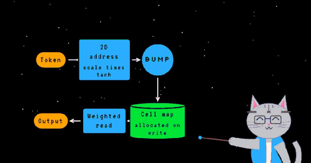
One μLattice layer (src/mulattice/models.py, MuLatticeMixer) takes the hidden state $h_t$ (width 64), runs a width-4 causal depthwise conv over it, and computes six things per token:

a write address $a^k_t = s \cdot \tanh(W_a h_t) \in \mathbb{R}^2$ and a separate read address $a^q_t = s \cdot \tanh(W_{aq} h_t)$ , where $s$ is a fixed scale (96 for the capacity checkpoint);
a content key $\kappa_t$ and query $q_t$ (unit-normalised, 32 wide per head), a value $v_t$ ;
a decay $\alpha_t \in (0, 1)$ and a write gate $\beta_t \in (0, 1)$ per head.

The address carries routing only. The content key decides what is stored inside a cell. That split matters: two different keys can share a cell and still be told apart by their $\kappa$ .

The bump kernel: why it is nine cells

A continuous address has to become a set of integer cells, differentiably. μLattice uses a compact bump in each axis:

b(t) = \cos^2\!\left(\frac{\pi t}{3}\right) \text{ for } |t| \lt \tfrac{3}{2}, \quad 0 \text{ otherwise}

normalised over the cells it touches:

\varphi_z(x) = \frac{b(x - z)}{\sqrt{\sum_j b(x - j)^2}}

The support is an open interval of length 3, so it contains at most three integers. In two dimensions the weight is the product $\varphi_{z_x}(x)\,\varphi_{z_y}(y)$ : at most a $3 \times 3$ patch, nine cells. Both $b$ and its derivative vanish at $|t| = 3/2$ , so as an address moves under gradient, a cell's weight fades out smoothly instead of snapping off. The normalisation makes $\sum \varphi^2 = 1$ over the nine cells, so the kernel between two addresses, $D(q, k) = \sum_z \varphi_z(q)\varphi_z(k)$ , is exactly 1 when they coincide and falls to 0 once they are three cells apart. "Exactly nine" in the paper is "at most nine": at a half-integer coordinate one of the three weights is exactly zero. At an integer coordinate the weights are 0.943, 0.236, 0.236 per axis (measured, from the formula).

Cells are gated-delta states in a hash map

Each lattice cell holds one $32 \times 32$ matrix $W_c$ per head, zero until something writes to it. For each of the nine cells around the write address, with $\varphi_c$ its bump weight:

\bar v = \alpha\, W_c \kappa, \qquad W_c \leftarrow \alpha W_c + \beta \varphi_c\, (v - \bar v)\, \kappa^\top

That is the gated delta rule from Gated DeltaNet, applied per cell: read back what the cell currently predicts for this key, write only the residual. Re-writing a key with a new value overwrites it algebraically, which is why the forgetting protocol works at all. The read uses the other address:

o_t = \sum_{c \in \text{3x3}(a^q_t)} \varphi_c(a^q_t)\, W_c\, q_t

The reference implementation (lattice.py) is a Python dict keyed by integer (x, y). The training scan (sparse_scan.py, fastscan.py) computes every address up front, sorts the cell keys to give each distinct cell a dense id, and runs the recurrence either token by token or cell by cell. The repository's tests check that the dict, the token loop and the cell-parallel scan agree; I ran them on CPU and every check passed, including "batched scan == hash-map lattice, max diff 5.55e-17" (measured).

one head, one lattice · scale 5 → 13 × 13 = 169 cells

keys written24

query x0.35

query y-0.8

query weights φ (rows y, columns x) · Σφ² = 1

0.002

0.074

0.051

0.021

0.741

0.514

0.010

0.347

0.240

cells allocated: 111 of 169
keys per cell: 0.142
keys sharing a centre cell: 4 of 24
keys the query overlaps: 6 · strongest D(q,k) = 0.186

Drag on the grid or use the sliders to move the query. Shaded blue cells exist because some key wrote to them; everything else is never allocated. The nine orange cells are what the query reads, weighted by φ. Every query touches at most nine cells however many keys are stored; what grows is how many other keys share those cells. Key positions here are random, not learned, so the collision rate is the birthday-problem rate the trained model beats with its spread loss.

The widget runs the exact kernel from kernel.py. Add keys and two things grow: the cells that exist because something wrote to them, and the density. The query never reads more than nine cells; what changes is how many other keys share them.

Where this sits

Memory addressed by location, with a few locations touched per access, is an old idea:

Sparse distributed memory (Kanerva, 1988) writes each item to every hard location within a Hamming radius of its address. μLattice's 3 x 3 patch is the same instinct with a smooth, learned, 2D address.
Lattice memory (Goucher and Troll, arXiv 2107.03474) is the closest ancestor I found: "a differentiable random access memory module with $O(1)$ performance regardless of size", entries on lattice points, nearest neighbours found by the lattice's symmetry, kernel-interpolated. Its memory is parametric, trained into the weights.
Product-key memory (Lample et al., arXiv 1907.05242) and hashed n-gram tables are also parametric: a huge table learned in training, read sparsely at inference.
Titans (arXiv 2501.00663) and the linear-attention variants are in-context, but fixed-size: the state is learned at test time, its shape set at build time.
Spotlight is in-context and grows. μLattice is that.

So the design is Spotlight's, with SDM and lattice memory as precedents. μLattice contributes the open, runnable version and hard-won training notes (PAPER.md Section 5: density ceilings, learning-rate entry, an address-scale change that collapses recall from 0.96 to 0.13).

Claim 1: "7,280x fewer operations than attention"

PAPER.md, Section 4.3: "At T=131,072: attention performs 1.1 trillion key-query comparisons; μLattice performs 151 million cell accesses — 7,280× fewer operations." Both numbers reproduce, as $64T^2 = 1.0995 \times 10^{12}$ and $9 \times 128 \times T = 1.51 \times 10^{8}$ ; their ratio is 7,281.8, which is $T / 18$ (reasoned). The README calls the figure "measured head-to-head on the same GPU". It is a count, not a measurement.

The two sides are not counted in the same unit. $64T^2$ is attention's multiply-adds (2 heads, 32-wide scores, 32-wide value mix, causal half of $T^2$ , both ways). The lattice side counts a "cell access" as 128 operations, but a cell access multiplies a $32 \times 32$ matrix. Per token, per head, a write touches nine cells three times (read-back $W\kappa$ , decay, rank-1 update) and a read touches nine more once: $9 \times 2 \times 4 \times 1024 = 73{,}728$ multiply-adds per token (reasoned, from sparse_scan.py).

T = 131,072, one layer	attention	μLattice	ratio
PAPER.md's count	1.1 trillion	151 million	7,280x
multiply-adds	1.1 trillion	9.66 billion	about 114x

The second row is reasoned. It is still two orders of magnitude, and it grows linearly with $T$ , so the architectural point stands: past a break-even near 1,152 tokens, the lattice does less arithmetic and the gap keeps widening. But 7,280x overstates the 131K gap by a factor of 64, and below about a thousand tokens attention does less work.

one layer · d_model 64 · 2 heads · log scaleT = 128K tokens

attention, causal multiply-adds1.1T

μLattice, multiply-adds (9 write + 9 read cells)9.7G

μLattice, PAPER.md's count (9 × 128 per token)151M

sequence length T128K

PAPER.md’s ratio (T / 18): 7,282×
multiply-add ratio: 114×

Both lines are straight on a log axis but with different slopes: attention’s total grows as T², the lattice’s as T. Where they cross depends on what you count. Counting every 32 × 32 matrix the lattice reads and writes puts the break-even near 1,152 tokens, and the gap at 131,072 tokens at about 114×, not 7,280×. Neither count is wall-clock: the measured table in PAPER.md has attention faster at every length it ran.

Wall-clock goes the other way. The paper's own table, from results/cost_comparison.json (reported), has attention faster at every length: 381.0 ms against 1,184.8 ms at 131,072 tokens. The paper says so and blames the Python-level scan, which is fair. What it reads as evidence is the slope: attention's per-token time rises from 1.1 to 2.9 μs (2.6x) while μLattice's stays near 9 μs. Two notes on that:

Attention's per-token compute grew 128x over that range (1K to 131K) while its time grew 2.6x (reasoned). At d_model 64 a fused attention kernel is dominated by fixed overhead, not by the $T^2$ term. The flat-versus-rising comparison is real, but it is measured in the regime where attention is cheapest.
The script that produced cost_comparison.json is not in the repository. I could not check which SDPA backend ran (PyTorch's FlashAttention backend needs fp16 or bf16; the rest of the repository runs fp32) or what the "attn peak MB" column, 16,248 MB at 131K against 3,195 MB for the lattice, includes; taken at face value it is the one column in the file that favours μLattice, but a fused kernel holds nothing like that, so it most likely counts materialised scores or allocator slack. The README's "flat at 9.5–9.8 μs from 32K to 131K tokens while cells grew from 1,246 to 37,100" also does not match that JSON, whose rows run 6.8 μs at 32,768 tokens to 9.0 μs at 131,072 (measured, from the file), and the cell counts appear in no results file.

Claim 2: memory that grows, "no fixed capacity", no quadratic blowup

Per-token cost is $O(1)$ in stored state: that is structural, and the unit test "per-token cost flat as memory grows" passed on my CPU, 185.5 to 197.8 μs per token as cells grew from 9,494 to 293,795 (measured, the repository's own test, not a trained model).

Memory is $O(T)$ , the same order as attention's KV cache, with a much larger constant. One cell is 2 heads of $32 \times 32$ fp32, 8 KiB (reasoned, PAPER.md agrees). At 8,192 stored pairs the lattice held 7,703 cells, 63 MB (reported). A KV cache for the same 133,120-token sequence at this width is $133{,}120 \times 512$ bytes, 65 MiB (reasoned). They come out about even here only because the protocol spends 16 tokens on each pair. On the cost benchmark, 37,100 cells is 290 MiB against 64 MiB of fp32 KV cache at 131,072 tokens (reasoned).

"No fixed capacity" is the claim I would retract. The address is $s \cdot \tanh(\cdot)$ , which confines every coordinate to $[-(s+1), s+1]$ : a box of $(2s + 3)^2$ cells, 38,025 at $s = 96$ , which caps the lattice at 297 MiB (reasoned). The scale is fixed before training. LIMITATIONS.md says it plainly: "The address scale must be set in advance so that the expected key count does not exceed this density." Recall degrades above about 0.22 to 0.25 keys per cell (Section 5.1), so the trained checkpoint's working capacity is about 8,400 to 9,500 keys (reasoned). The 37,100 cells on the cost benchmark are 97.6% of that box (reasoned). The model code itself records the trade-off: an unbounded linear address "breaks routing" and held-out recall stays 0.000. PAPER.md's own route out is 3D addressing, 27 cells per token, which is untested.

So: the per-token compute is genuinely flat and the store is allocated on demand, but the capacity is a hyperparameter, exactly as a fixed state's is. It is a much bigger one.

Claim 3: recall 1.0000 at 8,192 pairs

The capacity protocol (tests/test_capacity.py) stores 8,192 distinct key/value pairs with 14 filler tokens before each, 133,120 tokens in all, then asks 1,024 queries and reads the answer at each query's separator token. The released checkpoint scored 1,024 of 1,024 (reported, results/test_capacity.json), and 1,023 of 1,024 on the dense version with no filler.

I tried to re-run it. The README says the acceptance tests want a CUDA GPU (about 5 s there), and on this shared 4-core CPU box neither the 131K protocol (stopped after 15 minutes) nor the dense one (stopped after 6) finished, with most of the time spent in the kernel rather than in arithmetic (measured). So the recall figures here are reported. What I could check is that the result file is internally consistent (1,024 queries, all four depth quartiles at 1.0, T = 133,120) and that the code it comes from reads answers causally, one pass, at the separator.

What does it measure? Associative recall over a closed vocabulary. Keys are 16,384 token ids; each sequence draws 8,192 of them and pairs them with random value ids. The pairings are fresh every sequence, so the model is not memorising answers. But the address is a function of the key token's embedding, and every one of the 16,384 key ids has been seen thousands of times in training. The model learns a place for each one. The collision numbers show it: 8.7% of 8,192 keys share a cell at 0.215 keys per cell (reported), against about 19% for keys dropped uniformly at random into 38,025 cells (reasoned, $1 - e^{-8191/38025}$ ). Learned placement beats the birthday rate by about two to one.

The training recipe then pushes on exactly that vocabulary. The curriculum climbs 64 to 8,192 pairs, polishes "at the exact evaluation distribution" (filler 14, 8,192 pairs) and re-samples "keys that still fail" with 1/p loss weighting. experiments/polish_capacity_weakkeys.py names them: 16 key ids out of 16,384 caused every residual error, and the script forces those keys into every batch. Checkpoints were selected on fresh probe seeds, not on the test seed, so this is not test-set leakage in the usual sense. It is fitting the closed key space until every key has a clean cell. That is legitimate for a capacity demonstration. It tells you nothing about keys the model has never placed: Section 5.8 notes that a 16,384-key vocabulary trained from random initialisation "did not escape chance-level loss", and the 131,072-pair setting Spotlight reports would need about 262K keys and an untested scale near 385.

Everything is single-run: capacity and forgetting on one checkpoint each, two seeds for real-text retrieval.

Claim 4: the bolt-on to a frozen Qwen3.5-4B

A reply asked to "put it in a real llm"; the author pointed to experiments/boltoneval.py. Section 4.8 attaches the frozen capacity checkpoint to a frozen Qwen3.5-4B. Each test document holds 2 to 10 entity-value facts (eval_bolt_on.py). Entity and value strings are hashed with blake2b into the lattice's synthetic key and value ids and written in. At the question, the lattice's 64-wide readout goes through a 10.8M-parameter MLP that emits 8 soft-prompt tokens in front of the question. Only that bridge trains.

condition, 400 trials	exact match
frozen model, question only	0.025
document pasted into context	1.000
lattice soft tokens	0.645
soft tokens from another case	0.015

(reported). The per-type breakdown explains the 0.645 completely. I tallied the case files (measured): in seed 999 the test condition gets 122 of 200, and 122 is exactly the number of colour, food, number and time cases, every one of them right; all 38 city and 40 password cases are wrong. Seed 7777: 136 of 200, against 137 closed-type cases. The value strings of those four types come from small fixed sets (15 distinct times, 27 numbers in seed 999) that also appear in training.

That is what the mechanism predicts. The lattice retrieves the value id perfectly (lattice retrieval 1.0000). The bridge learns to turn a readout of a value id into the answer string, and it can only do that for strings it was trained on. A fresh password hashes to an id the bridge has never decoded. The test isolates a learned lookup decoder, not long-context memory: with 2 to 10 facts per document, pasting the document into a 4B model's context scores 1.000.

Two baselines would say more. One: a Python dict from entity hash to value id, feeding the same trained bridge. Since the lattice's retrieval is already perfect, I expect that to score the same 0.645 (reasoned). Two: enough facts per document that pasting them in costs real context. The JSONs also record test_vs_floor_z: 0.0 while the paper says the z-tests "underflow (p < 1e-15)"; the effect is obviously real, the stored statistic looks like a bug. And PAPER.md Section 6 still lists "The mixer has not been successfully attached to a frozen pretrained language model" as a limitation two pages after the bolt-on section.

Claim 5: what was not tested

This needs to be in large type. μLattice has not been tested as an attention replacement in language-model pretraining. PAPER.md says so twice and LIMITATIONS.md again. Every result is a one-layer, 64-wide mixer on synthetic recall, needle retrieval and bigram retrieval from wikitext. On MAD's Copy task it scores 0.003, because content-addressed cells have no notion of position. Spotlight's blog reports language-model runs at 140M to 670M parameters; μLattice does not reproduce those, so the "barrier broken" framing rests on Percepta's results, not on this repository's.

What holds

claim	verdict
per-token cost independent of what is stored	holds; structural, and the scan tests agree
"7,280x fewer operations"	the count mixes units; about 114x in multiply-adds at 131K, and slower in wall-clock
"quadratic memory barrier"	attention's memory is linear; the barrier is compute
"no fixed capacity"	does not hold; a tanh box of 38,025 cells, sized before training
recall 1.0000 at 8,192 pairs	reported, not re-run; a closed vocabulary the model was polished on
bolt-on 0.645 vs 0.025	holds; matches the share of test answers seen in training
LM pretraining	not tested

I like this repository more than its launch post. The scan code is careful, the tests check invariants, and the design constraints are negative results few people publish. If Spotlight's idea gets checked outside Percepta, it will be on code like this. The next experiments are cheap: a dict-plus-bridge baseline, keys outside the training vocabulary, and the mixer inside a small LM.