Linear attention's memory problem: four answers in one week

2026-10-06 · 20 min · linear-attention · attention · long-context · architecture · kv-cache · explainer

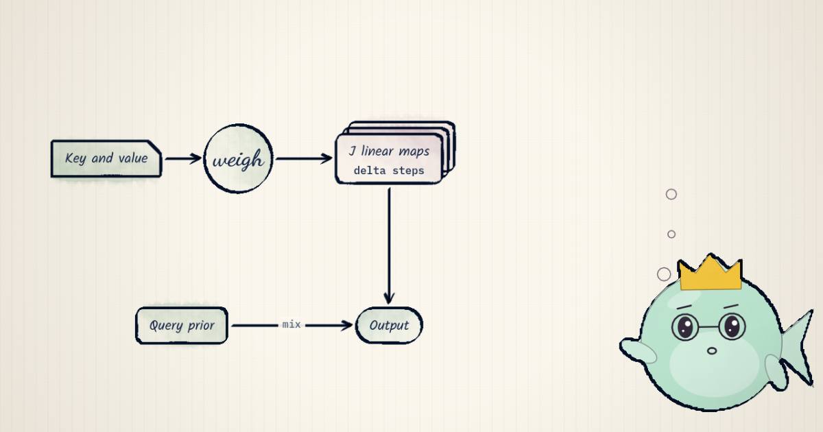
Softmax attention keeps every key and value it has seen. Linear attention keeps one matrix. Everything in between is an argument about what that matrix should be. In the first week of October 2026 four answers to that question landed in my feed at once:

SwiLA, Switching Linear Attention (arXiv 2609.39034, COLM 2026, code), from Scott Linderman's lab at Stanford.
Triadic linear attention, and Triadic Gated DeltaNet (arXiv 2609.36529, kernels, training code), from MIT and MIT-IBM.
Native Hybrid Attention, NHA (arXiv 2510.07019, code). It is a year old and had a new round of attention this week.
Spotlight Memory from Percepta (blog, companion post). It has no paper.

They look like four unrelated tricks. They are four edits to one object, and the object has a name.

The regression view

Wang et al.'s test-time regression framing, which the SwiLA paper builds on, says a sequence layer does two things at every token. It memorizes by fitting a function $m_t$ to the key/value pairs it has seen so far:

m_t \approx \arg\min_{m \in \mathcal{M}} \sum_{i=1}^{t} \lVert v_i - m(k_i) \rVert^2

and it retrieves by evaluating that function at the query, $o_t = m_t(q_t)$ . A layer is then two choices: the function class $\mathcal{M}$ and the optimizer that fits it online. The state is whatever the optimizer must carry from one token to the next.

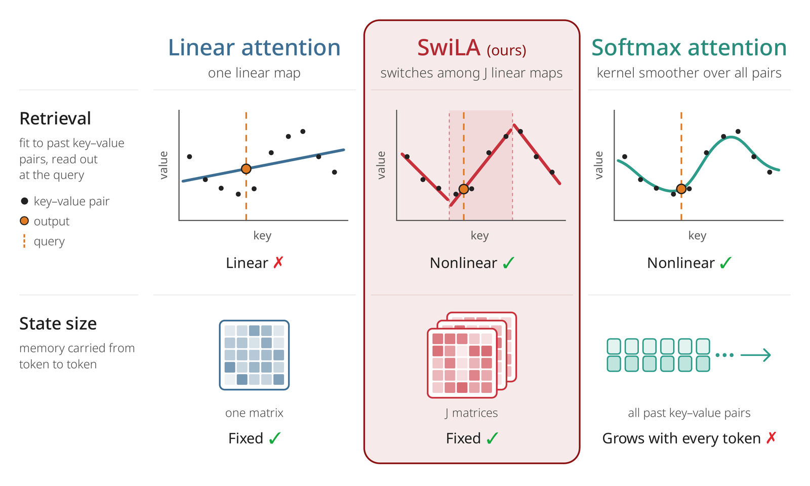
Three columns. Linear attention fits one straight line through scattered key-value points and keeps one matrix. SwiLA fits a piecewise-linear zigzag and keeps J matrices. Softmax attention fits a smooth curve and keeps every past key-value pair, a row that grows with every token. — The regression view in one picture: retrieval is a fit to past key/value pairs read out at the query, and the state is what the fit carries. Linear attention keeps one linear map, SwiLA switches among J of them, and softmax attention keeps every pair (SwiLA repository README, overview figure).

Three familiar layers fall out of three choices.

Softmax attention is a nonparametric kernel smoother. It does not fit weights at all. It stores every pair and weights them at read time by $\exp(q^\top k_i)$ . The state is the whole history: $2d$ numbers per token per KV head, growing forever. That is the KV cache; the attention-and-KV-cache explainer counts it byte by byte.

Linear attention fits a linear map $S$ , and its update is a Hebbian sum:

S_t = S_{t-1} + v_t k_t^\top, \qquad o_t = S_t q_t

The least-squares answer for a linear map is $S = (\sum v_i k_i^\top)(\sum k_i k_i^\top)^{-1}$ . Linear attention keeps the first factor and drops the inverse, which is exact only when the keys are orthonormal. With $d$ -dimensional keys there are at most $d$ orthonormal directions, so a $d \times d$ state stores at most $d$ associations cleanly. Past that, every readout picks up every other value in proportion to how much its key overlaps the query.

DeltaNet takes one gradient step on $\tfrac{1}{2}\lVert S k_t - v_t \rVert^2$ instead:

S_t = S_{t-1} + \beta_t \,(v_t - S_{t-1} k_t)\, k_t^\top

It subtracts what it currently predicts for $k_t$ before writing, so a key that gets a new value has its old value replaced rather than summed with it. Gated DeltaNet multiplies $S_{t-1}$ by a decay $\alpha_t$ first; in regression terms that is weight decay on the fast weights. The decay sets a memory half-life, which I worked through for Kimi's channel-wise version in KDA has a half-life, and the LTC and gated-delta piece derives the same recurrence from a liquid time-constant ODE.

Here is that difference in a toy I wrote for this piece. Sixteen-dimensional random sign keys and values, $N$ pairs written, optionally followed by new values for half the keys, then every key queried. A hit is a readout nearest the latest value written under that key.

toy recall · 16-dim keys and values · β = 0.5

then rewrite half the keys with new values (16 more writes)

linear attention (Hebbian)state 16 × 16 = 256 · 31.8%

DeltaNet (delta rule)state 16 × 16 = 256 · 49.2%

triadic delta, E = 4state 16 × 4 × 16 = 1024 · 93.5%

delta, 64-wide keystate 64 × 16 = 1024 · 96.1%

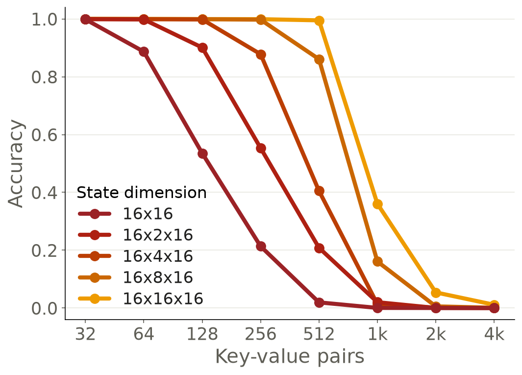
Recall rate over every key, averaged across 12 seeds. With the rewrite on, the Hebbian sum keeps both the old and the new value under a key and returns a blend; the delta rule subtracts what it predicted before it writes, so it returns the newer one. Neither fixes capacity: past about 16 pairs a 16-dim key space has run out of directions. The triadic joint key and a plain 64-wide key hold the same 1024 numbers and score about the same, which is the honest reading of the triadic paper: the gain is the bigger key space, and the trick is getting it from two small projections.

The numbers below are measured from that exact code (recall-sim.ts, 12 seeds, $\beta = 0.5$ ). At $N = 8$ with the rewrite, the Hebbian sum recalls 74.0% and the delta rule 96.9%: overwrites are the delta rule's job. At $N = 32$ with the rewrite, both have run out of room, at 31.8% and 49.2%. A memory holding a 64-dimensional key recalls 93.5% (triadic joint key) or 96.1% (a plain random 64-wide key). The update rule fixes interference. Only a bigger state fixes capacity.

That is the frame for the rest of this piece. SwiLA changes the function class. Triadic changes the state shape. NHA changes where exact memory lives. Spotlight changes whether the state is fixed at all.

The arithmetic first

Every number in this table is per head, per layer, and reasoned from the formulas each paper gives. I use $d = 128$ where a head dimension is needed.

design	what the state is	numbers kept	equals a KV cache of
softmax attention	every key and value	$2dT$	itself
linear attention, DeltaNet, GDN	one $d \times d$ map	16,384	64 tokens
SwiLA	$J$ maps of $d \times d$	$J d^2$	$J \times$ 64 tokens
Triadic GDN	one $d \times E \times d$ tensor	$E d^2$ (131,072 at $E = 8$ )	512 tokens at $E = 8$
NHA layer	$m$ key and $m$ value slots, plus a $w$ -token window	$2(m + w)d$ (24,576 at $m = 64$ , $w = 32$ )	$m + w$ tokens
Spotlight	a growing lattice of $d_k \times d_v$ cells	9 cells touched per token; total unreported	grows

Drag the head dimension, $J$ , $E$ , the window and the sequence length:

numbers kept per head, per layer · log scale

softmax KV cache 2·d·T8.39M numbers

linear attn / DeltaNet / GDN d²16k numbers · = KV cache at 64 tokens

SwiLA, J = 4 J·d²66k numbers · = KV cache at 256 tokens

triadic, E = 8 d·E·d131k numbers · = KV cache at 512 tokens

NHA, m = 64, w = 32 2·(m+w)·d25k numbers · = KV cache at 96 tokens

Spotlight, touched per token 9·d²147k numbers · = KV cache at 576 tokens · stored total: unreported

sequence length T32k tokens

SwiLA mixtures J4

triadic second key E8

NHA window w32

Every fixed-state answer equals some KV cache length: divide its numbers by the 2·d a cache stores per token. At d = 128 a DeltaNet head is worth 64 tokens of one KV head; a triadic head at E = 8 is worth 512. These are per head, so a model with grouped-query attention, which shares one KV head across several query heads, moves the crossover further out. The SwiLA row uses one d for every mixture; the paper instead shrinks each mixture’s d so that J·d² matches a DeltaNet budget.

The last column is the useful one. A fixed state is a promise to do as well as a KV cache of some length, and the crossover is short. A 400M-parameter Gated DeltaNet in the triadic paper carries 6.3 MB of state across 24 layers (reported, Table 1). The matched Transformer, with eight query heads per KV head, grows 12.6 MB per 1k tokens. The two are equal at 512 tokens (reasoned). The paper's PG19 figure marks that crossover and shows the GDN's loss falling behind the Transformer around 10k tokens.

SwiLA: change the function class

SwiLA replaces one linear regressor with a mixture of $J$ linear regressions. Each output coordinate $d$ of each value picks a component $j$ with a learned prior $\pi_{jd}(k_t)$ . Fitting a mixture online is online expectation-maximization, and one EM step per token gives the recurrence:

w_{tjd} = w_{t-1,jd} + \beta_{tjd}\, r_{tjd}\, \delta_{tjd}\, k_t, \qquad \delta_{tjd} = v_{td} - w_{t-1,jd}^\top k_t

It is a delta-rule step for every component, scaled by the responsibility $r_{tjd}$ : the posterior probability that component $j$ produced this coordinate, computed from the prior and from how small each component's prediction error is. Retrieval mixes the components with a query-side prior, $o_{td} = \sum_j \pi_{jd}(q_t)\, w_{tjd}^\top q_t$ . With $J = 1$ the responsibility is 1 and this is DeltaNet. Because each coordinate chooses on its own, the paper counts $J^D$ effective mixtures for $J D^2$ weights.

Panel A shows linear, switching and nonlinear regression fits to the same points. Panel B shows block diagrams of linear attention with one W matrix, SwiLA with a router choosing among three W matrices, and softmax attention over a growing grid of key-value cells. Panel C plots test R-squared against recurrent state size from 2^10 to 2^15, with SwiLA's red points above DeltaNet's blue points at every size. — SwiLA's three panels: why switching regression helps, the layer as a router over J matrices, and how well each layer imitates a softmax attention head at matched state size (SwiLA paper, Figure 1).

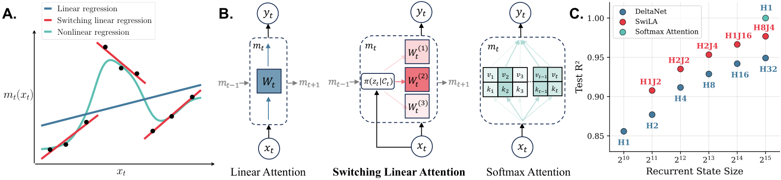
The cost is in that responsibility. It depends on the current state through $\delta$ , so the recurrence is nonlinear in its state, and the chunkwise-parallel trick every modern linear-attention kernel relies on does not apply. The authors train SwiLA sequentially with a recurrent Triton kernel. Their appendix sketches a way out: linearized, each parallel Newton iteration has DeltaNet's rank-one form and could reuse DeltaNet's chunkwise algorithm. It is not built yet.

Reported results, all at 374M parameters and 15B FineWeb-Edu tokens, with every recurrent model at the same 131,072 state numbers per layer. I checked that budget against the released config (swila_374M.json: 8 heads, expand_k 0.5 on a 1,024 hidden size, 4 experts, so $8 \times 4 \times 64 \times 64$ ; measured).

model	recall avg (6 tasks)	commonsense avg
Transformer++	28.3	45.3
DeltaNet	17.3	43.7
Gated DeltaNet	19.2	45.0
KDA	20.3	46.6
Gated Temporal SwiLA	20.6	45.4
Hybrid GDN (3:1)	29.5	44.3
Hybrid Temporal SwiLA (3:1)	31.8	45.1

The author's thread says every SwiLA variant beats DeltaNet on commonsense and recall. That holds in the tables. Read the margins, though. Against KDA, the best pure-recurrent baseline, the best SwiLA variant is 0.3 points ahead on recall and 1.2 behind on commonsense. The clearer win is in the hybrid, 31.8 against 29.5. The cleanest evidence is synthetic: on context-dependent recall, where the same key maps to different values under different context tokens, Temporal SwiLA is the smallest model to reach near-perfect accuracy, at a state of $2^{12}$ numbers. The speed bill is reported too: about 2x slower to train than GDN and 1.25-1.5x slower at inference, though still 4-5x the Transformer's end-to-end inference throughput at 1.3B.

Triadic: change the state shape

Linear attention got from a vector state to a matrix state with an outer product of two vectors. The triadic paper takes one more outer product. Each token also emits a small second key $k'_t$ and second query $q'_t$ of size $E$ . The write is the outer product of all three, the read contracts both key axes:

S_t = S_{t-1} + k_t \otimes k'_t \otimes v_t, \qquad o_t = \sum_{s \le t} (q_t^\top k_s)(q'^\top_t k'_s)\, v_s

The state is $d \times E \times d$ . With $E = 1$ and $k' = q' = 1$ it is ordinary linear attention. Flatten $\kappa_t = k_t \otimes k'_t$ and it is Gated DeltaNet with a $d \cdot E$ -dimensional key, read with $q_t \otimes q'_t$ . In regression terms the function class is still linear; what changed is the feature map. Orthonormal keys now come in $d \cdot E$ directions, not $d$ . In my toy the triadic memory and a plain 64-wide key score the same, 84.0% each at $N = 64$ without rewrites (measured). That is the paper's argument in miniature: the extra capacity comes from a bigger key space, and two small projections are a cheap way to buy one. $E = 8$ adds 1.2% to the parameter count (reported).

Line chart of recall accuracy against the number of key-value pairs from 32 to 4k. A 16x16 state falls off first, near 64 pairs. Each larger state, 16x2x16 through 16x16x16, holds full accuracy to roughly twice as many pairs as the one before. — Capacity in isolation: every doubling of the second key E shifts the recall curve right by about a doubling of key-value pairs, on a deliberately minimal two-layer model with no gating or delta rule (triadic paper, Figure 1).

The hard part is the kernel. At $E = 8$ one head's state is 512 KiB in FP32, twice a Hopper SM's register file (reported; $128 \times 8 \times 128 \times 4$ bytes is 524,288, reasoned). The authors tile each head along its value axis into 32-column blocks, one per thread block, so no SM ever holds the whole state. The Kronecker structure keeps the intra-chunk attention at $C \times C$ : it costs $C^2(d + E)$ instead of $C^2 d E$ .

Loss difference from a Transformer on PG19 against context position up to 64k. Gated DeltaNet starts below the Transformer and crosses above it near 10k tokens. Triadic GDN with E=2 crosses much later, and E=4 and E=8 stay below the Transformer all the way to 64k. Dashed vertical lines near the origin mark where the Transformer's KV cache outgrows each state. — Loss minus the Transformer's on PG19 books by context position, at 400M parameters: below zero is better. The dashed lines mark where the Transformer's cache passes each model's state (triadic paper, Figure 2, top left).

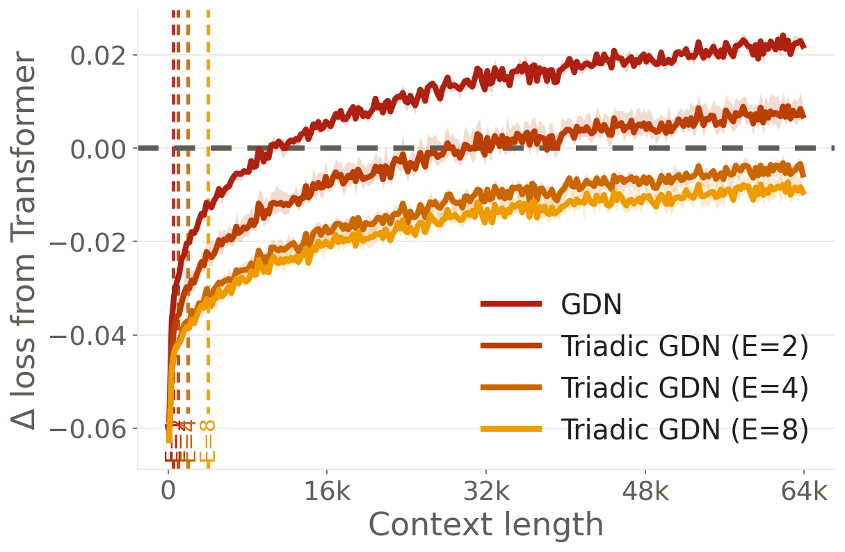
The reported state-matched comparison is the strongest evidence in this roundup, because the baselines spend the same state differently. At 4x GDN's state, with parameter count matched:

400M, 25.2 MB state	PG19 16k-64k ppl	recall avg
GDN base (6.3 MB)	14.15	26.2
larger heads, d = 512	14.24	28.5
grouped values, 4 per key	14.36	27.3
wider values, $d_v$ = 512	14.44	27.5
Triadic, E = 4	13.79	31.1
Transformer (cache grows)	13.92	41.6

I reproduced the state column from the training config (triadic_gdn_e8_400m.py: 24 layers, 8 heads of 128, second_key_dim 8). $24 \times 8 \times 128 \times 8 \times 128$ numbers at 2 bytes is 50.3 MB, the E = 8 figure in Table 2 (measured from the config, reasoned arithmetic). At E = 8 trained from scratch, recall reaches 33.1 against the Transformer's 41.6, so the gap narrows and stays open, as the first author's thread itself says.

The thread's "~15% for 4x more state" holds. Section 3.5 measures 14-15% over a FlashQLA TileLang GDN for $E = 4$ and 28-30% for $E = 8$ . Those are per-block forward-and-backward timings on one H100. In the hybrid experiment, making the GDN layers triadic beat doubling the attention layers' KV heads on perplexity and NIAH, trailed it by 0.8 on recall, and used about half the memory at 64k (220 MB against 407 MB).

NHA: change where the exact memory lives

NHA keeps two memories per layer and reads both with one softmax. Long-term memory is $m$ key slots and $m$ value slots, updated by a gated recurrence in the style of Gated Slot Attention: $K^{\text{long}}_t = \mathrm{Diag}(\alpha_t) K^{\text{long}}_{t-1} + (1 - \alpha_t) \otimes k_t$ , and the same for values. Short-term memory is the last $w$ tokens, kept exactly. The query attends over all $m + w$ keys at once, so the softmax itself decides, per query and per head, how much weight goes to the summary and how much to the window. A token shift keeps the two disjoint: only tokens leaving the window are written into the slots.

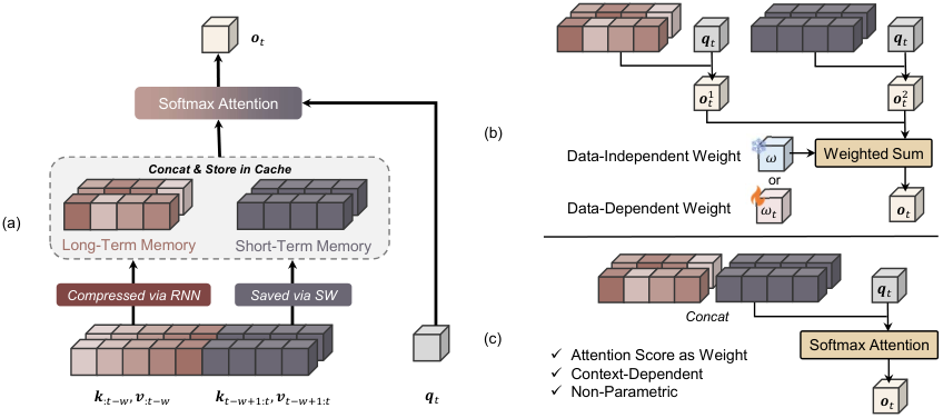
Diagram. Keys and values older than the window are compressed by an RNN into long-term memory slots; recent keys and values are saved by a sliding window into short-term memory; both are concatenated and read by one softmax attention with the query. Inset b shows prior hybrids computing two outputs and mixing them with a weight; inset c shows NHA's single softmax over the concatenation. — NHA's layer: RNN-compressed slots and an exact sliding window concatenated under a single softmax, against the usual two outputs and a learned mixing weight (NHA paper, Figure 2).

In regression terms NHA keeps softmax's function class, a kernel smoother, but smooths over a fixed budget of $m + w$ pairs: $w$ real ones and $m$ learned summaries. Its knob is the window. $w = 0$ is a pure linear RNN layer; $w$ equal to the sequence length is full attention. The released config defaults to 64 slots and a 32-token window (configuration_nha.py; measured), which the paper's ablation also picks as best.

Reported, at 340M parameters and 15B tokens: recall average 38.60 for NHA against 31.70 for Transformer++, 32.25 for the GDN hybrid and 36.97 for the GSA hybrid. At 1.3B and 100B tokens: 46.43 against 37.31 and 44.99. Two caveats the post does not mention. First, every hybrid in that table, NHA included, inserts one full-attention layer per eight, so none of them has a fixed total state; the comparison is hybrid against hybrid. Second, results come from one run with seed 42. The ablation is the convincing part: replacing the unified softmax with a learned weighted sum of two separate attentions drops recall from 38.60 to 33.59.

Spotlight: let the state grow, keep the access fixed

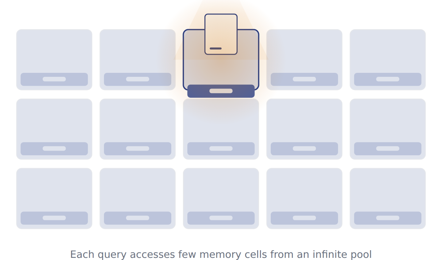
Percepta's answer refuses the premise. Spotlight maps every key and query to an address in a 2D lattice of cells. Each cell is a $d_k \times d_v$ DeltaNet state. A key writes to the cells around its address, and a query reads from the cells around its own. A cell is allocated the first time something writes to it. So memory grows with what has been written, and the work per token does not.

The addressing is made differentiable with a compact bump. In one dimension, $b(t) = \cos^2(\pi t / 3)$ for $\lvert t \rvert \lt 3/2$ and zero outside, so a real-valued address spreads its weight over the three nearest integer cells. In 2D the kernel is the product of two such bumps: every read and every write touches exactly $3 \times 3$ cells. The blog motivates it as a compact approximation to the RBF kernel that softmax attention computes for equal-norm keys. Routing runs on a 2D part of the key; the content lives in a separate high-dimensional part handled by the cell's delta rule.

A three by five grid of identical memory cells, each drawn as a card. One cell in the top row is highlighted with a glow and a page being written into it; the rest are dim. — Spotlight's lattice: each query touches a few cells from a pool that grows as keys write new addresses (Percepta, Spotlight Memory blog, lattice figure).

In the regression frame, my reading, labelled reasoned: this is SwiLA's piecewise-linear idea with the pieces allocated on demand. Each cell is a local linear regressor, the 2D address decides which ones a pair trains, and the bump interpolates between neighbours at read time. That is closer to local linear regression than to a mixture with a fixed $J$ .

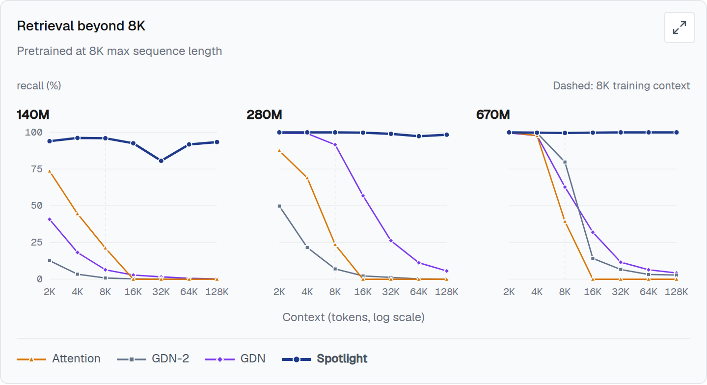
The reported numbers are striking. On MQAR with $2^{17} = 131{,}072$ pairs (a 524K-token context), Spotlight recalls 0.999, attention 1.000 and Gated DeltaNet 0.005. When half the keys are rewritten, Spotlight keeps 0.998 and attention drops to 0.748, because both values stay in its history. On RULER's single needle, models trained at 8K reach 93-100% at 128K for Spotlight and at most 5.6% for the fixed-state baselines. Short-context quality is level with the recurrent baselines, not better: at 670M the held-out loss at 8K is 2.154 against GDN's 2.142, and the lm-eval average is 33.1 against GDN's 34.1.

Three line charts of RULER single-needle recall from 2K to 128K context at 140M, 280M and 670M parameters. Spotlight stays near 100% across the range at every size, apart from a dip to about 80% at 32K for 140M. Attention, GDN and GDN-2 fall towards zero beyond the 8K training length. — Single-needle recall beyond the 8K training length; Percepta's own runs, not reproduced here (Percepta, Spotlight Memory blog, retrieval chart).

What I can and cannot check:

No paper, no LM checkpoints, no training code. The blog does not give $d_k$ , $d_v$ , head counts, token budgets, how many cells a trained model allocates per token, or wall-clock numbers. None of the language-modeling results can be re-run.
Attention's 0% beyond 16K is a length-extrapolation failure, not a capacity result. Those models were trained at 8K, and the chart's caption says attention scores 0% at 16K-128K with or without position rescaling. Spotlight extrapolating where attention does not is a real result; it is not evidence that attention runs out of memory.
The storage bill is open. Each write opens at most 9 new cells. If every token landed on fresh cells, a head would grow by $9 d_k d_v$ numbers per token, far more than a KV cache's $2d$ (reasoned). The real growth depends on how often addresses collide, and that is the number I would most like to see.
The Python demo is hand-built. The companion post says so: the interpreter was "hand-constructed" inside Spotlight. I read the released percepta-ai/spotlight-vm on Hugging Face through its safetensors headers (measured): the intelligence module is 47,192 float64 parameters, 45,830 of them in matrices, with d_model 16, 8 layers and 8 heads, which squares with the post's "under 100K matrix parameters". The core memory file holds 1,964,650 cells, each a 2-value entry at an integer $(x, y)$ address, in 24 MB. I could not reconcile that file with the post's diagram label of more than 100M memory parameters. The demo shows what such a memory can express. It does not show that training finds it.

A reply under the launch post linked arXiv 2605.30202 as related work. It is a dual-path looped-transformer paper from a different group, not Spotlight's.

Four edits, side by side

	edit, in regression terms	parallel training	state per head, $d = 128$	evidence
SwiLA	function class: mixture of $J$ linear maps	no, sequential for now	$J d^2$ , matched to GDN in the paper	374M, one budget, code released
Triadic GDN	feature map: $d \cdot E$ key from two projections	yes, chunkwise CuTe kernels	$E d^2$	400M and 1.3B, 3 seeds, state-matched baselines
NHA	kernel smoother over $m$ summaries plus $w$ exact pairs	yes, Triton kernel	$2(m+w)d$ plus 1 full layer in 8	340M and 1.3B, single run
Spotlight	growing set of local regressors, 2D addressed	not stated	grows; 9 cells read per token	blog only

What I take away

The triadic result is the one I trust most and the least surprising. It confirms that, at matched parameters, state size buys recall and long-context loss, and that how you spend the state matters: three standard ways of quadrupling it barely moved recall, and the Kronecker key moved it five points. If you are building a hybrid like Kimi K3's or Rigel's, the hybrid table says a bigger linear state can buy more than a bigger KV cache, for less memory at long context.

SwiLA is the most interesting idea and the least finished system. A nonlinear readout from a fixed state is exactly what the regression view says linear attention lacks, and the synthetic results show it. At 374M the language-model gains over KDA are within a point, and the sequential recurrence is a real tax until the Newton-iteration kernel exists.

NHA is a well-engineered hybrid, and its useful lesson is small: read both memories with one softmax rather than mixing two outputs. It belongs next to MiniMax's sparse attention and the Mamba family as a way of deciding which tokens stay exact.

Spotlight asks the right question. A fixed state, whatever its shape, is a KV cache of some fixed length, and a long enough sequence beats it. Constant work per token with a growing memory is the property worth having. Until there is a paper with the cell dimensions, the allocation rate and a model I can run, it is a claim with good charts.