2026-10-06 · 19 min · linear-attention · state-space-models · long-context · kv-cache · architecture · open-source · explainer
On 1 October 2026 BlinkDL announced RWKV-7 G1k: "100% RNN", "better every month", with a demo at rwkv.com and weights at BlinkDL/rwkv7-g1. Two days later he quoted his own post with a stronger claim:
Pure RNN is the safest SI approach too. All reasoning happens within its constant-size state (61x64x4096 = 16M numbers for RWKV-7 13B), without any growing KV cache. The tiny state is its whole mind (inner world model) suitable for all investigations
Three things are packed into that. An architecture: a recurrent layer whose memory is a fixed matrix per head. An arithmetic claim: that memory is 16 million numbers for the 13B model. And an opinion: a mind that small is the safe kind. I want to take them in that order, because the third only makes sense once the first two are pinned down, and the second is the only one I can check exactly.
Sources: the RWKV-7 "Goose" paper (arXiv 2503.14456), the
RWKV-LM repository at commit 20be0f8, the
Albatross inference repository at 545dd18, and the checkpoints
themselves. I did not run the models. Every number below is labelled measured (I read it from a file),
reported (someone else's figure) or reasoned (my arithmetic on the other two).
- task
- text-generation
- library
- rwkv
- license
- apache-2.0
- largest file
- 26.54 GB
- files
- 14
- downloads
- 25.8K
- likes
- 231
- languages
- en, zh, fr, es, de, pt
repo last modified 2026-09-30
What shipped
The Hugging Face repository holds four G1k checkpoints, all dated 20260930 and all named ctx25600
(measured, from the file list):
| file | size on disk | layers | width | heads | parameters |
|---|---|---|---|---|---|
rwkv7-g1k-1.5b-…pth | 3.06 GB | 24 | 2,048 | 32 | 1,527,668,736 |
rwkv7-g1k-2.9b-…pth | 5.90 GB | 32 | 2,560 | 40 | 2,948,065,280 |
rwkv7-g1k-7.2b-…pth | 14.40 GB | 32 | 4,096 | 64 | 7,199,932,416 |
rwkv7-g1k-13.3b-…pth | 26.54 GB | 61 | 4,096 | 64 | 13,270,298,624 |
I did not download 50 GB to get those shapes. A .pth file is a zip archive whose data.pkl entry lists every
tensor's name and shape, so three HTTP range requests per file (the zip's central directory, the local header,
then the pickle) recover the full table. I unpickled it with a loader that refuses every class except the tensor
rebuild function, so nothing in the file executes. Layer count is the highest blocks.N index plus one, width is
the embedding's second dimension, and the head count is the first dimension of att.r_k, which is
[heads, 64]. Parameters are the sum over all tensors (measured).
What "G1k" means is also readable from the repository, once you look at its history rather than its README. The
G1 family ("GooseOne" in the model card) is one set of base models trained continuously and released as monthly
snapshots, and the letter is the snapshot. The commit log shows g1h on 10 July, g1i on 5 August, g1j on 31
August and g1k on 30 September, each upload followed by the deletion of an older letter (measured). The G1k
files are byte-for-byte the same size as the G1j files at every scale, so the architecture did not change; the
weights kept training (reasoned). The context length in the filename did change: ctx8192 for G1g,
ctx10240 for G1h, ctx16384 for G1i and G1j, ctx25600 for G1k (measured). I read that as the training
sequence length, which is how RWKV-LM names its checkpoints; the card does not spell it out.
The model card calls these "BASE models (pretrained with web/code/synthetic + instruction/chat/reasoning data)". In a reply under the post, BlinkDL put the 13B's training so far at "9.8T tokens", growing by "0.83T each month due to limited compute" (reported). That last clause matters for reading "better every month": the improvement is mostly more tokens through the same network.
The architecture in one figure
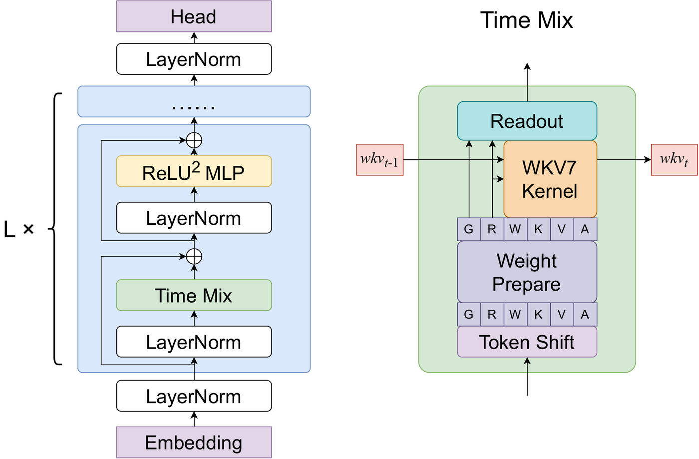
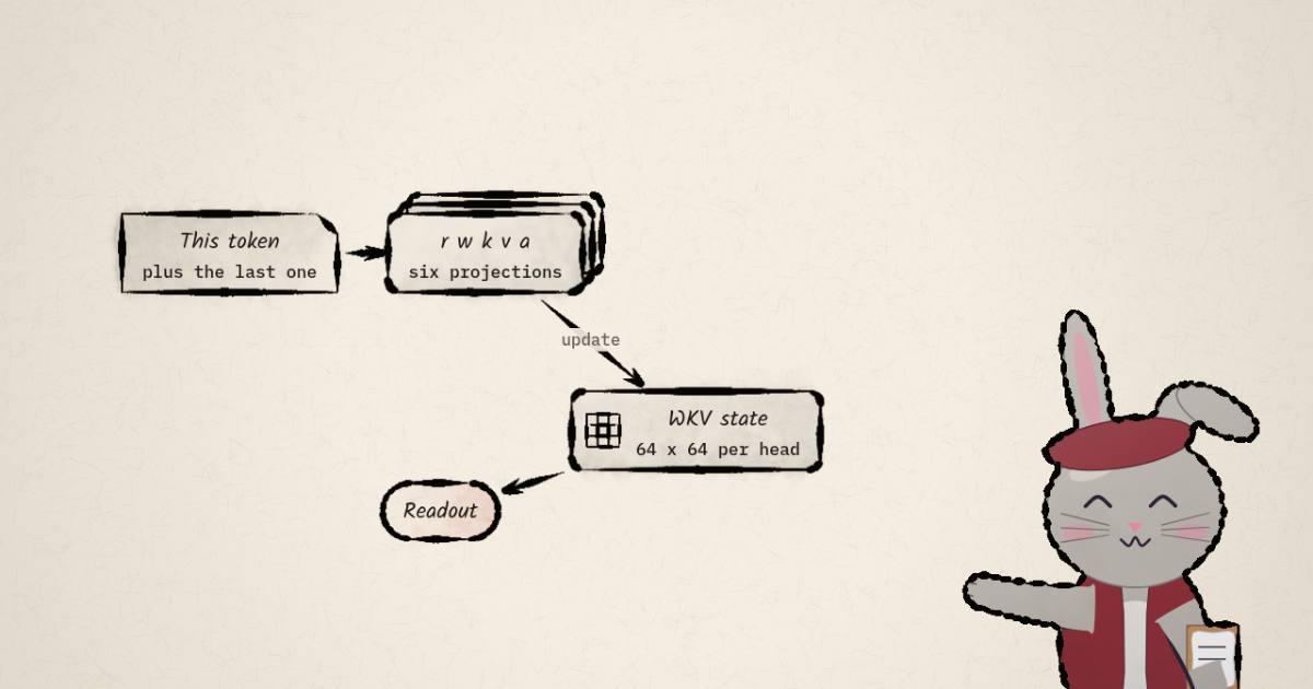
Each layer has two halves. The MLP is a plain two-matrix feed-forward with a squared ReLU and a hidden size four times the width. The time-mix half replaces attention. It first does a token shift: every projection's input is a learned per-channel blend of the current token's hidden vector and the previous one's . That costs one stored vector per layer. Then six projections come out: receptance (the query), decay , key , value , in-context learning rate and an output gate . The WKV kernel uses to update the state and to read it.
The interesting part is entirely in that kernel.
The state update from first principles
Start with linear attention. Drop the softmax and attention becomes a running sum of outer products: each token writes into a matrix , and a query reads . If the keys were orthonormal, reading with key would return exactly . That is a memory of fixed size, which is the point, and it has two problems. It never forgets, so the sum keeps growing. And when you write a new value at a key that is already in use, the old value stays: the read returns the sum of both.
Decay fixes the first problem bluntly. Multiply by a factor every step and old content fades. RWKV-6, Mamba-2, GLA and RetNet all do some version of this. The KDA half-life article works out how fast a per-channel decay forgets.
The delta rule fixes the second problem. Before writing at key , read what is already there, , and subtract it, scaled by a learning rate :
With and a unit key, the read at afterwards is exactly : the old value was erased and the new one written. This is one step of online gradient descent on , which is why the linear-attention roundup calls these layers test-time regressors. Gated DeltaNet multiplies in a scalar decay as well.
RWKV-7 generalizes three things. Written as the paper writes it, per head:
- Decay is a vector. has one entry per key channel, computed from the token, and each entry is restricted to , about , for stability.
- The learning rate is a vector. has one entry per channel, so the layer can replace some channels at a key and keep others. The paper calls it the in-context learning rate.
- The key you erase at is not the key you write at. The removal key is the key scaled by a learned vector and L2-normalized per head; the replacement key is the key blended toward .
The reference RNN code in RWKV-v7/rwkv_v7_demo_rnn.py is three lines once the projections are done:
# RWKV-LM @ 20be0f8, RWKV-v7/rwkv_v7_demo_rnn.py, time_mixing__
vk = v.view(H,N,1) @ k.view(H,1,N)                 # write: v k~^T
ab = (-kk).view(H,N,1) @ (kk*a).view(H,1,N)        # erase: -kappa^T (a * kappa)
state = state * w.view(H,1,N) + state @ ab.float() + vk.float()
out = state.to(dtype=x.dtype) @ r.view(H,N,1)      # read with receptance
state is [H, N, N] with N = 64: one 64 by 64 matrix per head. The paper's own picture of it is a 4 by 4
toy:

The widget below runs that update on a 4 by 4 head, with and as scalars and so they fit on sliders. It writes at , at an overlapping key (their dot product is 0.36), and then overwrites with .
- 1. write v₁ at key k₁
- 2. write v₂ at key k₂ (k₁·k₂ = 0.36, they overlap)
- 3. overwrite: write v₃ at key k₁ again
| read | y = S r | want | error |
|---|---|---|---|
| r = k₁ | [0.00, 0.00, 1.00, 0.00] | v₃ | 0.00 |
| r = k₂ | [-0.31, 0.87, 0.36, 0.00] | v₂ | 0.49 |
With a = 0 the overwrite stacks on top: reading k₁ returns v₁ + v₃ plus 0.36 of v₂. With a = 1 it returns exactly v₃, but the erase at k₁ also takes 0.36 of the overlap out of k₂’s slot. A fixed state stores cleanly only what its keys can keep apart.
With and (plain linear attention), reading after the overwrite returns plus 0.36 of : an error of 1.06 against the you wanted. With it returns exactly . But look at : erasing along also removed the part of 's slot that overlapped it, and the read at is off by 0.49 (linear attention is off by 0.51 there, for a different reason). A fixed matrix can only keep apart as many things as its keys can keep apart. A 64-wide head has 64 orthogonal directions; everything beyond that shares space (reasoned, from the toy).
Two properties of the transition matrix are the paper's main theoretical claims (reported, proved in its appendix). Its eigenvalues stay in , so the state cannot blow up. And because is not diagonal and depends on the input, a stack of these layers can track state in ways a diagonal-decay RNN or a transformer cannot under standard complexity assumptions: the paper proves that a 4-layer RWKV-7 can recognize any regular language, and that one layer solves the permutation-tracking problem. That is the strongest technical sense in which "reasoning happens in the state" is more than a slogan: the state is not a passive buffer, it is the register of a finite automaton the network can learn to run.
Asked under the post about Kimi Delta Attention, BlinkDL replied: "It's a weaker (and slightly faster on GPU) form of the general DPLR RWKV-7 design… GDN => KDA => RWKV-7". DPLR is diagonal plus low rank, which describes all three transitions: Gated DeltaNet uses a scalar decay and one key, KDA a per-channel decay and one key, RWKV-7 a per-channel decay, a per-channel learning rate and separate erase and write keys (reasoned, from the three update rules). "Weaker" in the sense of strictly fewer degrees of freedom per step is fair; whether that shows up in quality at equal compute is an empirical question nobody in that thread answered. The liquid time-constant article traces the same recurrence back through another literature.
Counting the 16 million
The post's arithmetic is . From the checkpoint: 61 layers, 64 heads, and each head is a matrix, which is 4,096 numbers. So
That is 15,990,784 WKV numbers (measured shapes, reasoned product). The 4,096 in the post is the head's matrix, not the model width, which happens to also be 4,096 on this model. "16M" is right.
It is not quite the whole state. Token shift keeps the previous token's hidden vector twice per layer, once for time-mix and once for the MLP: , which is 499,712 more numbers. The full recurrent state of the 13.3B model is 16,490,496 numbers (reasoned). The paper's table of released models lists state size as "WKV + Shift" in exactly this form, and its rows for the 1.5B (3,145,728 + 98,304) and 2.9B (5,242,880 + 163,840) match what I get from the G1k checkpoints at those sizes (measured against reported).
How many bytes that is depends on the runtime. RWKV-LM's reference RNN allocates the WKV state in fp32 and the
shift vectors in the model dtype; Albatross, BlinkDL's fast inference engine, keeps all of it in fp16
(measured, from the torch.zeros calls in each). For the 13.3B that is 62.0 MiB in the reference layout and
31.5 MiB in fp16 (reasoned).
| model | layers x heads | state numbers | reference (fp32 WKV) | fp16 |
|---|---|---|---|---|
| G1k 1.5B | 24 x 32 | 3,244,032 | 12.2 MiB | 6.2 MiB |
| G1k 2.9B | 32 x 40 | 5,406,720 | 20.3 MiB | 10.3 MiB |
| G1k 7.2B | 32 x 64 | 8,650,752 | 32.5 MiB | 16.5 MiB |
| G1k 13.3B | 61 x 64 | 16,490,496 | 62.0 MiB | 31.5 MiB |
Against a KV cache
A transformer's equivalent is the KV cache: for every token, every layer stores a key and a value per KV head.
The cleanest comparison is the Qwen3 family, which sits in the same leaderboard and publishes its shapes. From
each model's config.json (measured), every Qwen3 dense model uses 8 KV heads of dimension 128, so the cache
per token is numbers: 81,920 for Qwen3-14B's 40 layers, 160 KiB
in bf16.
Divide and the crossover is early. The 13.3B's 16,490,496 state numbers equal Qwen3-14B's cache at 202 tokens; in bytes, with the reference fp32 state, at 397 tokens (reasoned). At G1k's own training length of 25,600 tokens the Qwen3-14B cache is 3.9 GiB against 31.5 MiB, about 127 times larger. At tokens it is 160 GiB, more than six times the 26.54 GB the 13.3B's weights take on disk (reasoned). Qwen3-14B's config lists a 40,960-token native window, so the million-token row is a hypothetical for that particular model; the per-token rate is not. A multi-head-attention model is worse: Llama-2-13B, with 40 KV heads, stores 409,600 numbers per token, five times Qwen3's (measured from its config).
- state numbers
- 61·64·64·64 + 2·61·4096 = 16,490,496
- KV numbers per token
- 2·40·8·128 = 81,920
- equal in numbers at
- 202 tokens
- equal in bytes at
- 397 tokens
- cache ÷ state at this length
- 82.6x
The RWKV bar does not move with the context slider; that is the whole claim. The KV bar crosses it within a few hundred tokens for every size, and by a million tokens a 14B-class cache is larger than the 13.3B model’s own weights. What the bars do not show is what each memory can hold: the cache keeps every key and value exactly, the state keeps whatever the update rule decided was worth keeping.
Batch size multiplies both, which is where the constant state pays off in practice. Albatross reports "10250+ token/s RWKV-7 7.2B fp16 bsz960 decoding @ RTX5090 (always const speed & vram)" (reported). At 16.5 MiB per sequence in fp16, 960 sequences of state is 15.5 GiB, next to about 14.4 GB of weights: consistent with one 32 GB card (reasoned). The same batch of a transformer at any useful context would not fit.
Now the other side of the ledger, which the bars cannot show. A KV cache is lossless: whatever was in token 3 is still there, exactly, at token 300,000. A fixed state is lossy by construction; the widget above already shows two overlapping keys interfering at dimension 4. The paper is candid about this. On its passkey test, "RWKV7-World3-1.5B achieves perfect accuracy up to a context length of 19600 tokens but exhibits degradation beyond 20600 tokens", and the 2.9B holds "perfect retrieval up to 35000 tokens" before degrading (reported). And on long books, the World-trained 2.9B's loss starts climbing past about 10K tokens:
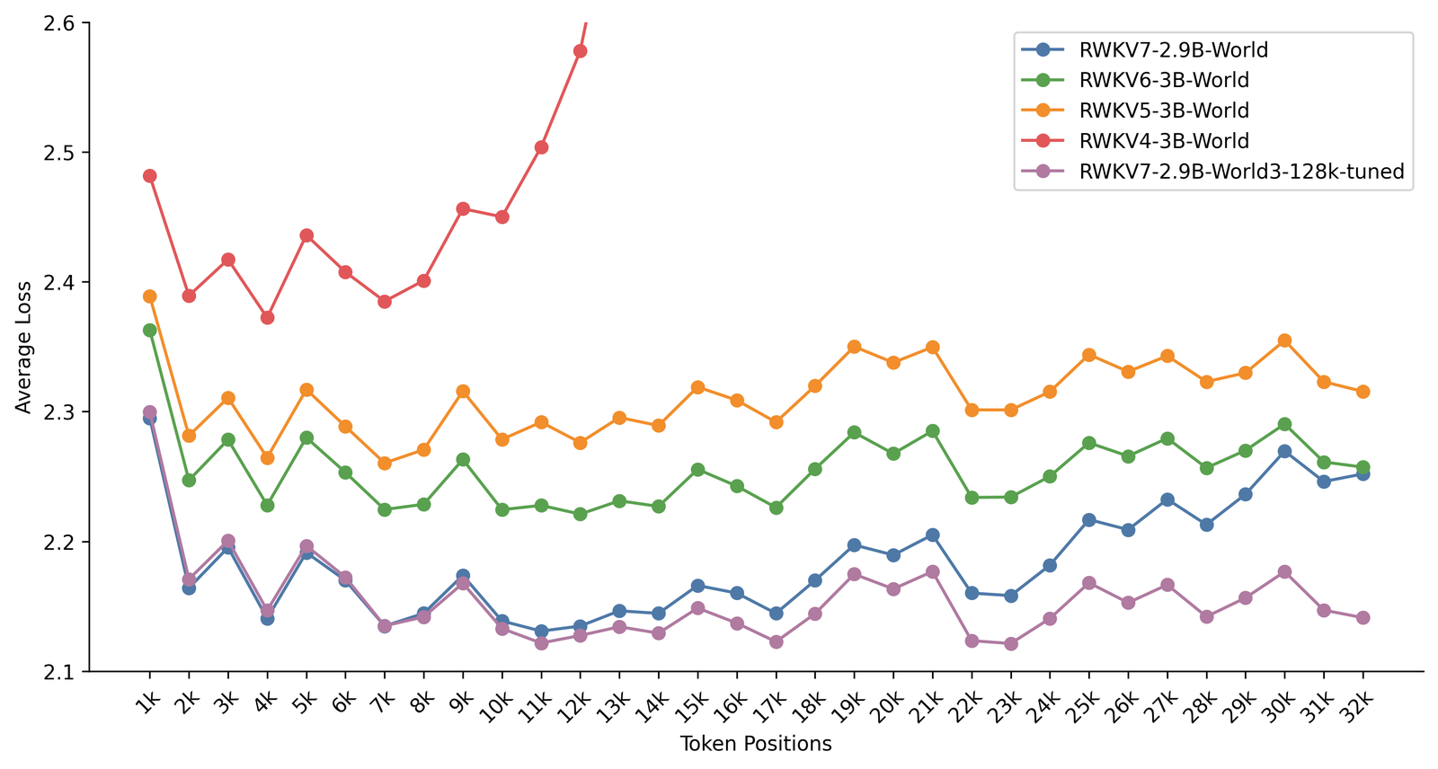
The paper attributes that rise to overfitting to the 4K pretraining length and shows long-context fine-tuning removes it. The G1 line has been pushing training length up every few months, to 25,600 for G1k, which is the same remedy applied continuously. I have no long-context measurement for G1k itself; none was posted.
What "better every month" measured
The release image is a screenshot of UncheatableEval, a leaderboard that scores base models by how well they compress text published after their training cutoffs (lower is better; the image does not name the unit, and compression ratio is the first of the metrics the leaderboard's code offers).
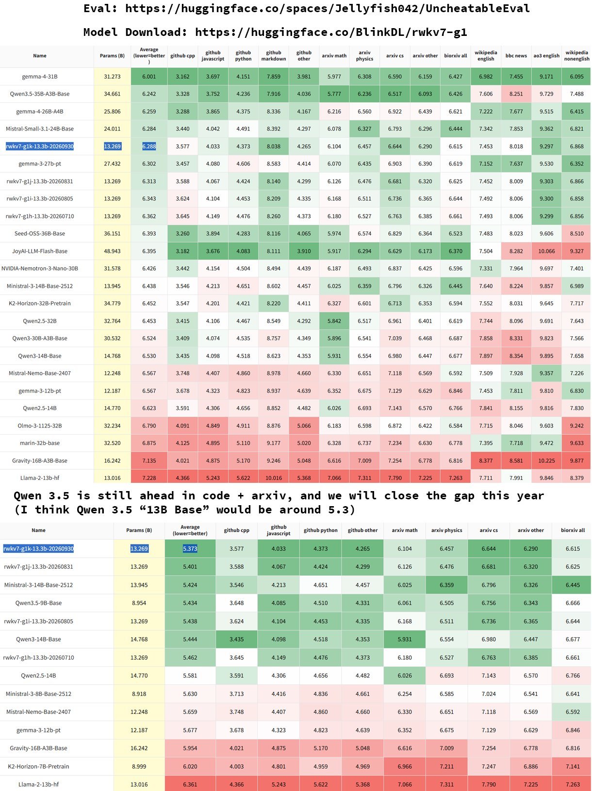
Read off the image (reported): the 13.3B scores 6.288 for G1k, 6.313 for G1j, 6.343 for G1i and 6.362 for G1h, so the monthly steps are 0.019, 0.030 and 0.025 (reasoned). G1k lands between Mistral-Small-3.1-24B (6.284) and gemma-3-27b (6.302), behind gemma-4-31B (6.001) and Qwen3.5-35B-A3B (6.242), all of them larger. On the lower table, which keeps only models up to about 16B and only the code, arXiv and bioRxiv columns, it leads at 5.373, ahead of Ministral-3-14B (5.424) and Qwen3.5-9B (5.434). BlinkDL's own caption concedes the gap: "Qwen 3.5 is still ahead in code + arxiv".
Three cautions on reading this. It is a compression benchmark of base models, so it says nothing directly about chat, tool use or reasoning; the model card links a GPQA evaluation script but the release posted no such number. The lower table is a subset of models and columns chosen by the publisher; it is not wrong, but it is the flattering cut. And "better every month" is literally true on this metric for four consecutive releases, at a cost of about 0.83T tokens a month.
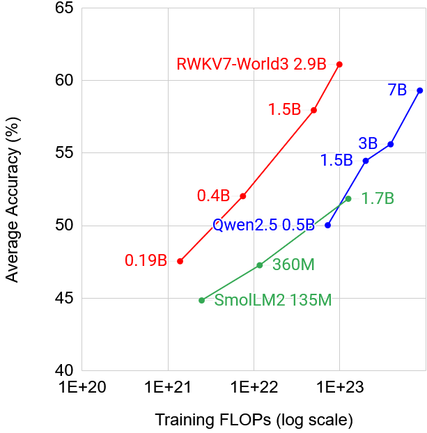
For the architecture itself, the paper's headline evidence is older and on smaller models: trained on far fewer tokens than its peers, RWKV7-World3 traces a better accuracy-per-FLOP curve on multilingual benchmarks than Qwen2.5 and SmolLM2 (reported).
The safety claim, calmly
"The safest SI approach" is an opinion, and the post does not argue it beyond the size of the state. It is worth separating what in it is true, what is overstated, and what could be tested.
What is true. Everything an RWKV-7 model carries from one token to the next is a fixed-size object you can copy, save, diff, restore and edit. For the 13.3B, 16,490,496 numbers; in fp16 that is at most about 33 million bytes of information per sequence, no matter how long the sequence runs (reasoned). That is a hard ceiling a transformer does not have, and it is an operational convenience as well: you can checkpoint a conversation as 31.5 MiB, fork it, or roll it back. The ecosystem already edits states directly; RWKV-PEFT, which the model card links for training, lists "State Tuning" next to LoRA, which learns an initial state instead of new weights.
What is overstated. "All reasoning happens within its constant-size state" is true of what persists across tokens, not of computation. The reasoning on any single token happens in 13.3 billion weights, and the state is only the thread between steps. A transformer's KV cache is also a complete, finite, inspectable record of everything the model carries forward; it is bigger, and it grows, but it is not less transparent. And a model that writes a chain of thought carries part of its "mind" in the emitted tokens, which it reads back as input, for an RNN as for a transformer. 16 million numbers is small next to a 160 GiB cache, but it is not small next to what interpretability tools currently explain; nobody can read a 16M-dimensional vector as a world model yet.
What is testable. Each of these would turn the opinion into evidence, and none needs anything beyond the released weights:
- Probes. Train linear probes on the WKV state to recover facts about the context: which entities were mentioned, a board position, a variable's value in code. The paper's appendix already trains small RWKV-7 models on Reversi and reports they learn board state tracking before evaluation; a probe on the state would show where that board lives.
- Interventions. Patch one head's 64 by 64 matrix from another context and see whether the downstream behaviour changes the way the probe predicts. If editing the state reliably edits beliefs, "the state is its whole mind" earns its keep.
- Capacity. Measure how recall degrades with the number of distinct facts held, against the 64-direction ceiling per head the toy above illustrates. That bounds what any long-horizon plan can keep without writing it down.
If those come back clean, a bounded, editable state is a real advantage for oversight over a cache that grows without limit. If they come back like most interpretability results, it is an advantage of degree.
What I would take away
The 16M figure is right, and checkable from the checkpoint without running it: 61 layers, 64 heads, 64 by 64 per head, plus half a million numbers of token shift. The update that fills that state is a delta rule made per-channel in both forgetting and learning, with separate keys for erasing and writing, and the paper's expressivity results are about exactly that structure. Against a same-size transformer the state is the size of a few hundred tokens of KV cache, which is why RWKV serves hundreds of sequences on one consumer GPU. The price is that the memory is lossy, and the long-context curves show it. The safety argument is an interesting hypothesis about oversight, not a result; the experiments that would settle it are cheap, and the weights are Apache-2.0.