Liquid time constants and gated delta rules: two literatures, one recurrence

2026-08-10 · 14 min · linear-attention · state-space-models · attention · math · explainer · open-source

There are two separate research literatures about neural networks that forget at an input-dependent rate, and as far as I can tell they mostly do not read each other.

One starts in continuous time. Liquid Time-constant Networks (Hasani, Lechner, Amini, Rus and Grosu, 2020) are ODEs, motivated by the neural dynamics of C. elegans, analysed with stability theorems and solved with numerical integrators. The other starts in discrete time. Gated DeltaNet (Yang, Kautz and Hatamizadeh, 2024) is a linear attention variant, motivated by retrieval failures in efficient Transformers, analysed through online learning and implemented with chunkwise GPU kernels.

They are the same recurrence. Not analogous — the same. This piece derives that correspondence from each paper's own equations, works through what each tradition figured out that the other did not, and then reads LTCAttention, an implementation published today that sits deliberately between them.

Part 1 — What "liquid" means

A plain continuous-time RNN decays toward its input at a fixed rate: $dx/dt = -x/\tau + S(t)$ , where $\tau$ is a learned constant. Every input, every timestep, same $\tau$ . LTC's move is to let the decay rate be a function of the state and the input. Substituting $S(t) = f(\mathbf{x}(t), \mathbf{I}(t), t, \theta)(A - \mathbf{x}(t))$ gives the paper's Equation 1:

\frac{d\mathbf{x}(t)}{dt} = -\left[\frac{1}{\tau} + f(\mathbf{x}(t), \mathbf{I}(t), t, \theta)\right]\mathbf{x}(t) + f(\mathbf{x}(t), \mathbf{I}(t), t, \theta)\,A

Read the bracket. The coefficient multiplying $\mathbf{x}$ is the decay rate, and it now contains $f$ — a neural network. So the system time constant is

\tau_{\text{sys}} = \frac{\tau}{1 + \tau f(\mathbf{x}(t), \mathbf{I}(t), t, \theta)}

which is a number the network computes fresh at every point in time from whatever it is currently looking at. That is the whole idea, and the name: a time constant that flows.

liquid time constant · τ_sys = τ / (1 + τ·f)arXiv 2006.04439, Eq. 1 & Thm. 1

τ/(1 + τW) = 4.8τ_sys = 33.3 stepsτ = 100

the whole interval — Theorem 1 says the time constant can never leave it, however large the input grows

state decay with no new input · x(t) = e^(−t/τ_sys)

t = 0dashed line = half the signal gonet = 200

input drive f0.020

τ_sys

33.3 steps

effective time constant

α = e^(−1/τ_sys)

0.97045

one-step retention

half-life

23.1 steps

when half the signal is gone

A conventional RNN fixes its decay rate at training time. An LTC makes it an output of the network: a gate f reads the current state and the current input, and the answer sets how fast this neuron forgets on this timestep. Turn the drive up and the memory horizon collapses from 100 steps toward 5; turn it down and the neuron holds. The bounds matter as much as the mechanism — because f is a bounded sigmoid, the time constant is trapped in a finite interval no matter how extreme the input, which is what makes the system provably stable rather than merely usually stable.

The paper's two theorems are what make this more than a reparameterization. Because $f$ is a bounded sigmoidal nonlinearity, Theorem 1 traps the time constant:

\frac{\tau_i}{1 + \tau_i W_i} \le \tau_{\text{sys}_i} \le \tau_i

and Theorem 2 traps the state itself between $\min(0, A_i^{\min})$ and $\max(0, A_i^{\max})$ , "which guarantees that the outputs of LTCs never explode even if their inputs grow to infinity." Those are unusual guarantees. A model whose decay rate is an unconstrained network output could in principle be driven to instability by an adversarial input; LTC's cannot, by construction.

This is worth flagging because the same argument recurs, unattributed, throughout modern gated linear attention. Every one of these architectures constrains its gate — Mamba2 through a softplus and a discretization, Gated DeltaNet by requiring $\alpha_t \in (0,1)$ , Kimi K3's KDA through a gate_lower_bound on $\log\alpha$ . The reason is always the same one LTC proved in 2020: an unbounded forgetting rate is an unbounded system.

Part 2 — The bridge

Now the part neither literature states, which falls out of LTC's own Algorithm 1. Solving Equation 1 in closed form is not possible, so the paper introduces a fused solver — a semi-implicit Euler step that reads

\mathbf{x}(t + \Delta t) = \frac{\mathbf{x}(t) + \Delta t \, f(\mathbf{x}(t), \mathbf{I}(t), t, \theta) \odot A}{1 + \Delta t\left(\frac{1}{\tau} + f(\mathbf{x}(t), \mathbf{I}(t), t, \theta)\right)}

Look at the denominator. Writing $g$ for the gate output,

1 + \Delta t\left(\tfrac{1}{\tau} + g\right) = 1 + \Delta t\,\frac{1 + \tau g}{\tau} = 1 + \frac{\Delta t}{\tau_{\text{sys}}}

because $\tau_{\text{sys}} = \tau/(1 + \tau g)$ by definition. So the entire update is

\mathbf{x}_{t+1} = \bar{\alpha}\,\mathbf{x}_t + \bar{\alpha}\,\Delta t\, g \odot A, \qquad \bar{\alpha} = \frac{1}{1 + \Delta t/\tau_{\text{sys}}}

That is a gated linear recurrence. Previous state times a scalar in $(0,1)$ , plus a write. The scalar depends on the input, through $g$ . This is structurally identical to what Mamba2, Gated DeltaNet and KDA do — the object those papers call $\alpha_t$ and describe as a "data-dependent gating term."

The only difference is which approximation of the exponential you use. The exact solution of the linear ODE over a step decays by $e^{-\Delta t/\tau_{\text{sys}}}$ ; LTC's fused solver uses $1/(1 + \Delta t/\tau_{\text{sys}})$ , which is the $[0/1]$ Padé approximant of that exponential.

LTC fused solver vs. the gated-linear-attention conventionz = Δt / τ_sys

LTC · Algorithm 1

ᾱ = 1 / (1 + z)

0.952381

half-life 14.2 steps

exact ODE · GDN, Mamba2, KDA

α = e^(−z)

0.951229

half-life 13.9 steps

retention per step, as a function of zPadé overshoots by 0.12%

z = 0 · never forgetsz = 1.2 · forgets fast

z = Δt/τ_sys0.050

Take LTC’s fused solver step, group the terms, and the denominator collapses to 1 + Δt/τ_sys. What is left is a gated linear recurrence: last state times a scalar in (0,1), plus a write. That scalar is the thing Gated DeltaNet calls α and Mamba2 calls the decay gate — LTC just spells it as a Padé approximant of the exponential rather than the exponential itself. In the regime these models actually run in (small z, long memory) the two agree to a fraction of a percent. The literatures are not analogous. They are the same recurrence, discretized two different ways.

In the regime these models actually operate in — long memory, so $\Delta t \ll \tau_{\text{sys}}$ — the two agree to a fraction of a percent. LTC picked the Padé form because it is what makes the implicit Euler step solvable in closed form; the linear-attention literature picked the exponential because $\alpha^n$ composes cleanly across a chunk, which is what its parallel scan needs. Same recurrence, two discretizations, chosen for two different implementation reasons.

Which means the three quantities have one meaning:

tradition	symbol	this article's other coverage
continuous-time / LTC	$\tau_{\text{sys}}$ , a time constant in seconds	Part 1 above
gated linear attention	$\alpha_t = e^{-\Delta t/\tau}$ , retention per token	KDA has a half-life
what you should think in	$n_{1/2} = \ln 0.5 / \ln \alpha$ , a horizon in tokens	same

I have argued the third column before, and the LTC connection strengthens it: a half-life is just $\tau_{\text{sys}}$ in units a language model can be reasoned about in. $\tau$ , $\alpha$ and $n_{1/2}$ are one number in three coordinate systems.

Part 3 — What gating alone cannot do

If the story ended there, Gated DeltaNet would be LTC with better kernels. It is not, and the difference is the delta rule.

A gated linear attention state is a matrix $\mathbf{S}$ holding key-value associations. Pure gating updates it as $\mathbf{S}_t = \alpha_t \mathbf{S}_{t-1} + v_t k_t^\top$ : scale everything down, add the new pair. The problem the Gated DeltaNet paper identifies is that $\alpha_t$ is a single number multiplying the entire state. It can dump everything, and it can hold everything, and it has no way to express forget this one fact, keep the rest.

DeltaNet solved that with the delta rule, which subtracts the state's existing content at the current key before writing the new one — but, as the paper puts it, "since this process only modifies a single key-value pair at a time, the model lacks the ability to rapidly clear outdated or irrelevant information, especially during context switches." One mechanism clears the table but cannot pick up a single plate; the other picks up single plates but cannot clear the table.

The gated delta rule (Equation 8) is both terms in one product:

\mathbf{S}_t = \mathbf{S}_{t-1}\left(\alpha_t\left(\mathbf{I} - \beta_t k_t k_t^\top\right)\right) + \beta_t v_t k_t^\top

gated delta rule · S_t = S_t−1(α(I − βkkᵀ)) + βvkᵀarXiv 2412.06464, Eq. 8

survives · every direction ⊥ k90.0%

controlled by α alone — the global forgetting knob

survives · the direction along k27.0%

α(1 − β) — global decay AND targeted erasure

α 0.900β 0.70

both active — decay the whole state while overwriting this key harder than the rest.

The paper’s argument is that these two knobs are complementary rather than redundant, and the two bars are why. α is a blunt instrument: it scales everything the state holds, so it can dump a whole stale context at a topic switch but cannot forget one fact and keep the rest. β is a scalpel: it subtracts precisely the component along the key being written, so it can overwrite one association without disturbing anything else — but it can only ever touch one key per step, so clearing a long context takes as many steps as there were keys. DeltaNet had the scalpel and no way to clear the table; Mamba2 had the table-clearing and no scalpel. The gated delta rule is just both terms in the same product.

The two bars are the whole argument. Along any direction orthogonal to the current key, the surviving fraction is $\alpha_t$ — the global forgetting knob. Along $k_t$ itself it is $\alpha_t(1 - \beta_t)$ — global decay and targeted erasure. Set $\alpha_t \to 1$ and you have DeltaNet; set $\beta_t \to 0$ and you have Mamba2; the useful region is the interior.

Part 4 — LTCAttention, and a third place to put a time constant

Both traditions above put the time constant on a recurrent state. LTCAttention by Rikka Botan, published today under MIT, puts it somewhere else: on the attention score itself.

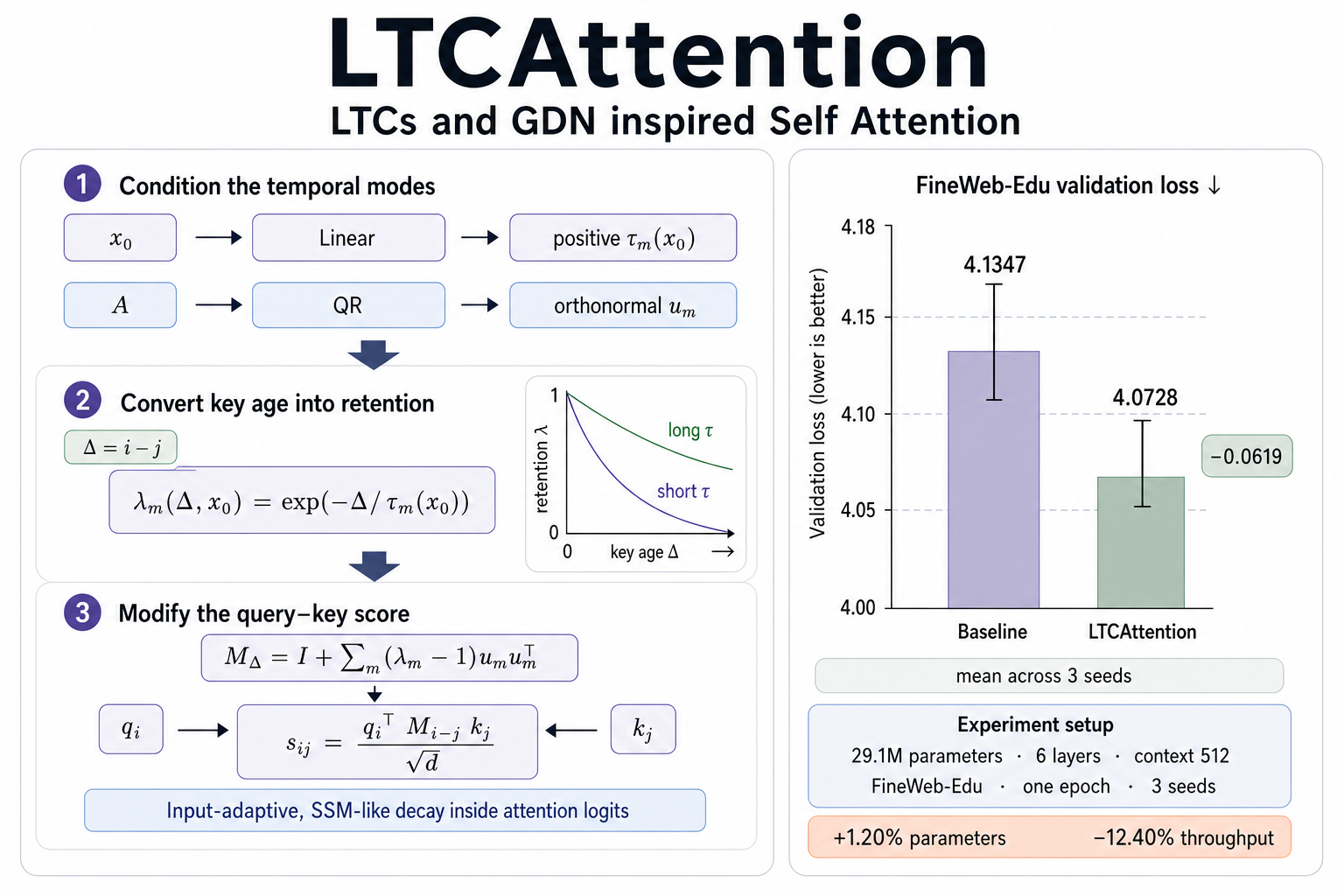
Overview graphic for LTCAttention showing input-conditioned time constants feeding learned orthonormal temporal modes, which form a time-varying Householder-form metric applied to query-key inner products inside causal self-attention. — LTCAttention's mechanism: input-conditioned time constants set per-mode retention, which enters causal attention as a metric on the query-key inner product (Rikka Botan, LTCAttention repository, 2026).

The construction is worth following because it is genuinely clever. Each KV head carries $M$ learned directions, orthonormalized by QR so that $u_m^\top u_n = \delta_{mn}$ . The first token of the causal block, $x_0$ , sets every mode's time constant through one linear projection:

\tau_{h,m}(x_0) = \frac{\tau_{\min}}{\sigma\!\left(r_{h,m} + \delta_{h,m}\right)} > \tau_{\min}

That is the LTC principle exactly — a positive, input-conditioned, bounded-below time constant, with the sigmoid playing the role LTC's Theorem 1 played. Because $x_0$ is visible to every position in the block, reading it keeps the controller causal.

For a query at $i$ and a key at $j \le i$ , with key age $\Delta = i - j$ , mode $m$ retains $\lambda_m(\Delta) = e^{-\Delta/\tau_m}$ , and the modes assemble into

M_\Delta(x_0) = \prod_{m=1}^{M}\left[\mathbf{I} - (1 - \lambda_m)u_mu_m^\top\right] = \mathbf{I} + \sum_{m=1}^{M}\left(\lambda_m(\Delta, x_0) - 1\right)u_mu_m^\top

which drops into the score as $s_{ij} = q_i^\top M_{i-j}(x_0)\,k_j/\sqrt{d}$ .

LTCAttention · λ_m(Δ) = e^(−Δ/τ_m) applied to the scoreτ_min = 512/12 = 42.7

score weight retained, by key age Δ = i − j

Δ = 0 · same tokenhalf retainedΔ = 512

fast mode

τ = 47

half-life 33 tokens

medium mode

τ = 95

half-life 66 tokens

slow mode

τ = 356

half-life 246 tokens

δ from x₀+0.00

Drag δ and every mode’s horizon moves together — that is the LTC principle, transplanted from a recurrent state onto an attention score. One linear projection of the block’s first token sets all the time constants, and because that token is visible to every query, the controller stays causal. The division by a sigmoid is what keeps it honest: τ = τ_min/σ(·) is always greater than τ_min, so no mode can decay arbitrarily fast and no exponent can blow up. The modes are orthonormal, so each one owns a direction in head space and decays independently — a spectrum of memory horizons inside a single head, exactly as in a per-channel gated linear attention, but expressed as a metric on the query-key inner product instead of a recurrent state.

The effect: the learned orthogonal complement passes through untouched, while each temporal mode is an eigenvector with eigenvalue $\lambda_m$ . Since $\lambda_m(\Delta) = a_m^\Delta$ with $a_m = e^{-1/\tau_m}$ , this is the same stable diagonal decay law as an SSM — just expressed as a metric on an inner product rather than a state update.

The factorization is the load-bearing trick, and it checks out

Applying a different $M_\Delta$ to every $(i,j)$ pair naively means building a $T \times T \times d$ object. LTCAttention avoids it by pushing the decay into the queries and keys separately, around a fixed center $c$ :

q_i' = q_i + \sum_m \left(e^{-\frac{i-c}{\tau_m}} - 1\right)(q_i^\top u_m)u_m, \qquad k_j' = k_j + \sum_m \left(e^{\frac{j-c}{\tau_m}} - 1\right)(k_j^\top u_m)u_m

I checked the algebra rather than taking it on faith. Decompose $q_i = q_\perp + \sum_m (q_i^\top u_m)u_m$ using orthonormality; the transform replaces each modal coefficient by $e^{-(i-c)/\tau_m}(q_i^\top u_m)$ and leaves $q_\perp$ alone, and symmetrically for $k$ . Their inner product is then

q_i'^\top k_j' = q_\perp^\top k_\perp + \sum_m e^{-\frac{i-c}{\tau_m}}e^{\frac{j-c}{\tau_m}}(q_i^\top u_m)(k_j^\top u_m) = q_\perp^\top k_\perp + \sum_m e^{-\frac{i-j}{\tau_m}}(q_i^\top u_m)(k_j^\top u_m)

and expanding $q_i^\top M_\Delta k_j$ directly gives the same thing. The center $c$ cancels, exactly as claimed. The modal projections cost $O(TMd)$ , so scaled dot-product attention remains the only quadratic operation — the mechanism is free at the asymptotic level and the standard SDPA kernel is still doing the heavy lifting.

There is a real numerical hazard hiding in that trick, and the code knows it. The factors $e^{-(i-c)/\tau}$ and $e^{(j-c)/\tau}$ are individually huge or tiny even though their product is bounded by 1; they cancel only algebraically. The implementation handles this two ways. It computes the exponents in FP32 or FP64 regardless of the BF16 activation dtype, with a comment saying exactly why. And it fixes $c$ at the middle of the context, centre = 0.5 * (max_positions - 1), rather than recomputing it per prefix — which both keeps cached keys valid as the KV cache grows and halves the worst-case exponent.

The choice of $\tau_{\min}$ then finishes the job, and this is my favourite detail in the repository. The default is min_tau = max_positions / 12. Combined with the centered origin, the largest exponent magnitude is

\frac{(T-1)/2}{T/12} = \frac{6(T-1)}{T} \approx 6

independent of context length. Whatever $T$ you configure, the factorization's intermediate values stay inside roughly $e^{\pm 6}$ . That is not a coincidence; it is a bound chosen so the trick cannot overflow.

The experiment, and the number that worries me

The repository ships a real controlled study rather than a claim: three seeds, a paired comparison, SHA-256 checksums on the tokenized data, one epoch over 287,588,352 FineWeb-Edu tokens consumed without replacement, and the full result JSON checked in.

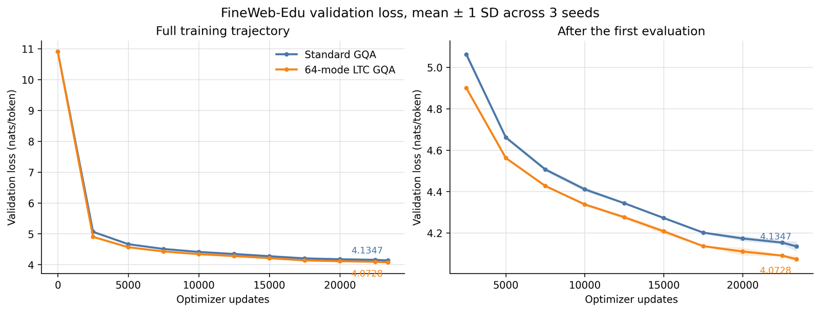
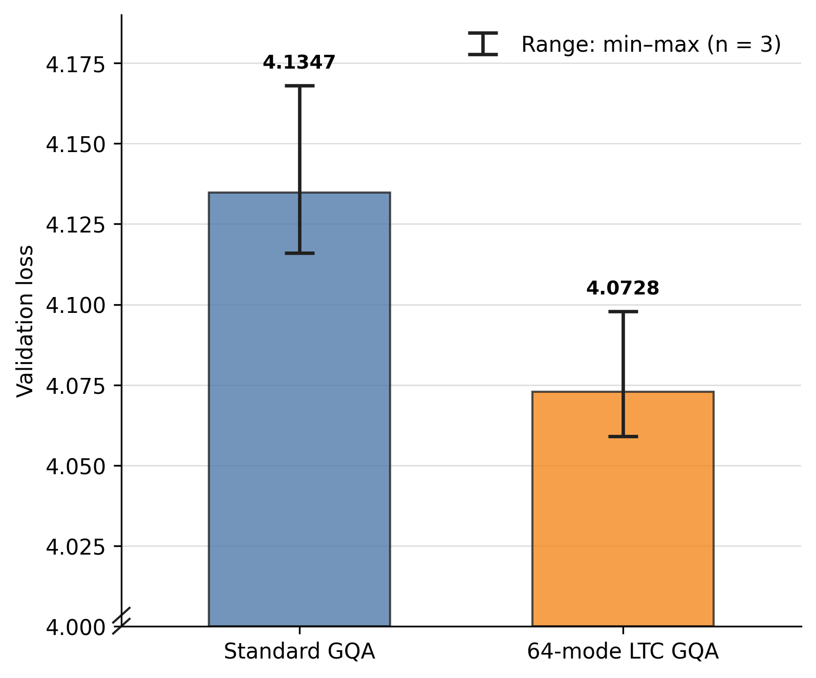
Validation loss curves over training for the LTC model and the standard baseline across three seeds, with the LTC curves sitting consistently below the baseline curves through the second half of training. — Validation loss across training, three seeds per variant (Rikka Botan, LTCAttention repository, 2026).

Final validation loss per seed for the LTC model and the standard baseline, showing the LTC variant lower in all three seeds with non-overlapping means. — Final validation loss by seed; LTC is lower in all three (Rikka Botan, LTCAttention repository, 2026).

Reading the numbers straight out of results/fineweb_edu_fullrank_29m_6layer_half_3seeds.json:

	validation loss	perplexity
standard	4.13471 ± 0.02367	62.49
LTC	4.07281 ± 0.01777	58.73
paired difference	−0.06190 ± 0.00646

The per-seed differences are −0.0544, −0.0702 and −0.0610 — negative in all three, with a spread ten times smaller than the effect. As a paired result at this scale that is about as clean as three seeds get, and the README is careful to say that "three seeds and one small model scale do not establish broad scaling behavior."

Two confounds are worth quantifying, and the repository reports exactly the numbers needed to do it.

Parameters. LTC adds 345,600 of them, +1.20%. Borrowing the Chinchilla-form sensitivity $\partial L \approx \alpha\,(A/N^\alpha)\,(\partial N/N)$ with $\alpha = 0.34$ , a 1.20% parameter increase at 28.8M is worth roughly 0.005 nats. The observed effect is more than ten times that. The gain is not just parameter count.

Compute. This is the one. LTC also runs 12.40% slower (142,473 vs 162,638 tokens/sec, measured and reported by the author). The comparison is token-matched, not wall-clock-matched. Spend that same 12.4% on more training tokens for the baseline instead, and the same scaling form ( $\beta = 0.28$ on the data term) predicts a gain of roughly 0.061 nats — which is, to two decimal places, the entire measured effect.

warning

I want to be precise about what that estimate is and is not. The coefficients come from a scaling law fitted on a different corpus, tokenizer and budget, so the absolute numbers do not transfer; I am borrowing only the sensitivity, and the error bars on that are wide. The near-exact agreement between 0.061 and 0.062 is a coincidence of a rough calculation, not a measurement. But the direction is robust: at this scale, a 12% throughput penalty buys enough extra tokens to be the same order as the observed quality gain. The missing experiment is a wall-clock-matched run, and until someone does it the honest reading is that LTCAttention is better per token and undetermined per second. That the author reported the throughput cost at all is what makes this check possible — most releases do not.

One further limitation, stated plainly in the repo: the released code is LTC-only, and the baseline artifacts are "retained only as experiment provenance." So the comparison cannot currently be re-run from this repository, only re-read.

What each tradition knows

Setting the implementations aside, the two literatures have complementary blind spots.

LTC knows about stability and it knows about time. It has proofs that the time constant and the state stay bounded under arbitrary input. It treats $\Delta t$ as a real quantity, which means it handles irregularly sampled sequences natively — a capability the discrete-time literature mostly gave up without noticing, because tokens arrive on a uniform grid. And it thinks in a unit, seconds, that forces you to ask how long a memory is supposed to last.

Gated linear attention knows about scale and it knows about writing. It has the chunkwise parallel algorithms that make these recurrences trainable on modern hardware at all, which is the entire reason the idea reached billion-parameter models. And it has the delta rule — a way to modify one association without disturbing the others that has no counterpart in the LTC formulation, where the "write" is just $f \cdot A$ added to a decaying state.

LTCAttention is interesting mostly as evidence that the gap is crossable in either direction: it takes LTC's bounded input-conditioned $\tau$ , GDN's adaptive retention, and applies them to a third substrate neither paper considered. Whether that particular hybrid pays for its 12% is, on the evidence available, not yet settled. Whether the two literatures should be reading each other seems to me much clearer.

Sources: Liquid Time-constant Networks (arXiv 2006.04439, Hasani, Lechner, Amini, Rus, Grosu) for Equation 1, Algorithm 1, and Theorems 1–2, read via ar5iv; Gated Delta Networks: Improving Mamba2 with Delta Rule (arXiv 2412.06464, Yang, Kautz, Hatamizadeh) for Equation 8 and the complementarity argument; and the LTCAttention repository at its 2026-08-10 state — README.md, model.py, config/, and results/fineweb_edu_fullrank_29m_6layer_half_3seeds.json. The three figures are LTCAttention's own, flattened onto white. The fused-solver-to-gated-recurrence derivation, the verification of the query-key factorization, the $\tau_{\min} = T/12$ bound, and both scaling estimates are mine and are shown in full above so they can be checked. All four interactives are mine.