2026-11-09 · 38 min · attention · long-context · sparse-attention · inference · kv-cache
Why read this
Hightop 30%How LSA's Ward buckets replace the key scan, the 98% recounted, and CPU ports of flat and tree that find the pooling and deep beams cost recall.
- Interactive explanations
- Original analysis
- A lasting reference
LLM architectureNeeds datacenter GPUsApache-2.0Research paper
How this was scored
- Is it new?
- 2 of 3: A real new idea, method or capability
- Can I trust it?
- 2 of 3: Measures key facts from files, code or configs
- Can I run it?
- 2 of 3: Open code or weights with real limits
- Will I understand it?
- 3 of 3: Mechanism carried by interactives built from real code or data
- Can I act on it?
- 2 of 3: A concrete recipe, numbers or comparison
- Will it last?
- 2 of 3: A reference for a year or more
- Does it affect many?
- 1 of 3: A specialist community
- Only here?
- 2 of 3: A teardown or measurement few others did
Score 72 of 100, ranked 105 of 701 rated articles. Each question is answered 0–3 by hand, and a 3 is rare. How articles are scored
Sparse attention has a dirty secret, and the Latent Sparse Attention paper puts it in its second figure. A sparse-attention layer reads only a few thousand keys per query, which makes the attention cheap. Something has to choose those keys, though. That something is the indexer, and in every production design I know of it still scores every preceding key, or every block of four keys, for every query. At 10M tokens, that scan is 98% of the layer's prefill time.
LSA, from Prefrontal AI and ETH Zurich (code at Prefrontal-AI/latent-sparse-attention, Apache-2.0), replaces the scan with a search. Keys are clustered by meaning into buckets of about eight. A query scores one centroid per bucket, keeps the best buckets, and attends to their keys. The attention kernel is unchanged; only the list of keys it reads is different.
I read the paper and the code (at commit 6291aa6), and I ported the reference flat and tree designs to numpy to see
how well bucket search finds the keys that exact scoring would have found, how much the tree gives up for scoring
fewer vectors, and whether the selection bill the paper measures on an H200 falls out of plain arithmetic. Every
number below is labelled: measured (I ran it), reported
(the paper or a post says so), or reasoned (my arithmetic or inference).
Where the time goes
Sparse attention splits a layer into two jobs. The indexer picks, for each query, a set of key positions. The attention then runs over only. With a fixed budget of keys, the attention costs to prefill a context of tokens and per decoded token. The indexer is the catch: if it scores every key, it is still in prefill and in decode, only with a smaller constant.
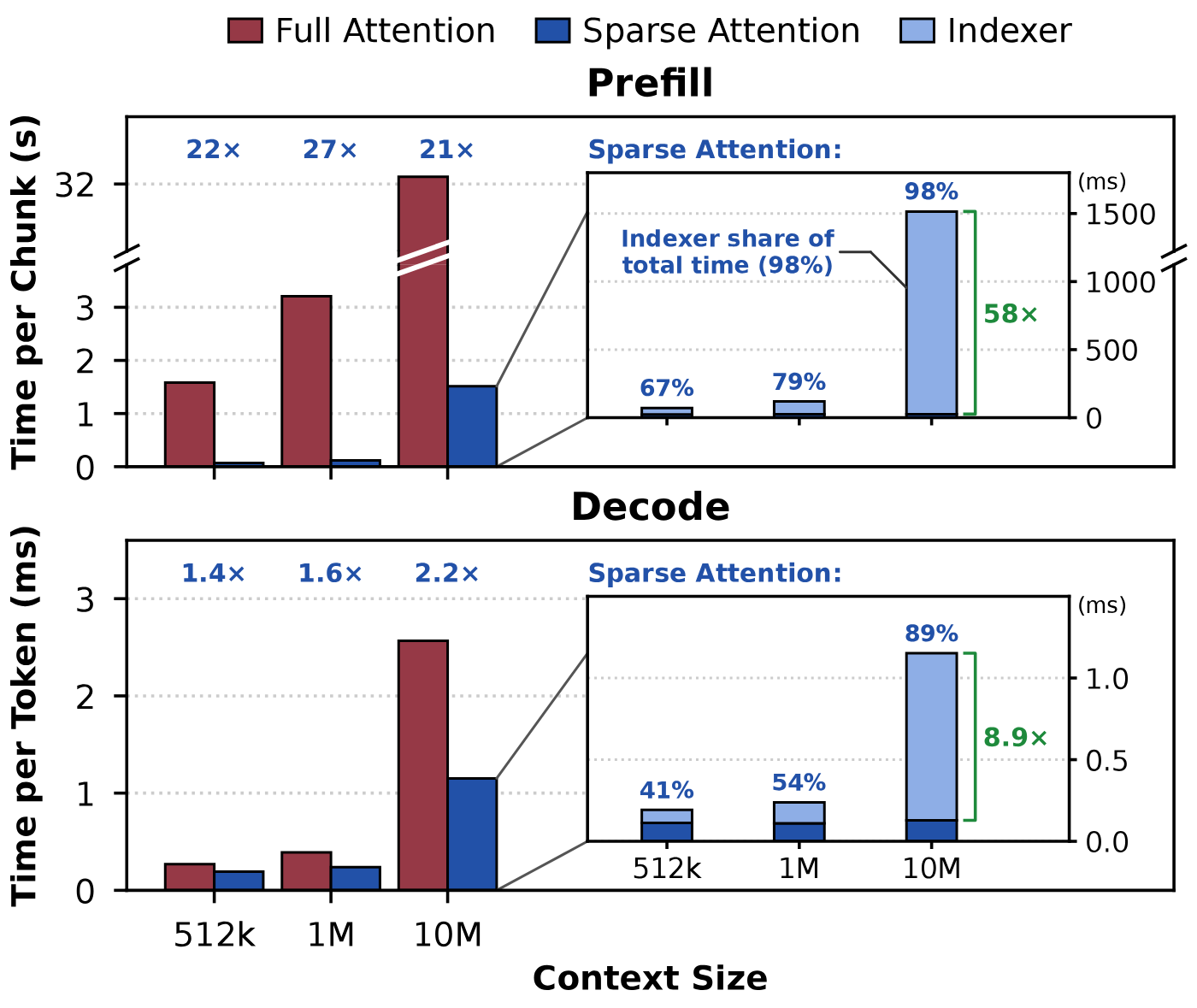
The paper's own numbers (reported): on GLM-5.3-Flash at 10M tokens, a free indexer would make its sparse
attention a further 58x faster in prefill and 8.9x in decode. The constant the indexer already saves is not small.
GLM-5.3-Flash's config.json (measured, read from the Hub) gives its indexer 32 heads of 128 dims, scoring keys
pooled four at a time: multiply-adds per query. Even that is a quadratic
bill at 10M tokens.
Two things in that widget matter more than the headline. First, the speedup is a long-context phenomenon: on
GLM-5.3-Flash, D-LSA is 2.1x faster per layer in prefill at 512k and 22.7x at 10M (reported). Second, a layer
is not a model. Qwen3.8-27B has 16 full-attention layers out of 64; the other 48 are linear attention
(measured, layer_types in its config.json). GLM-5.3-Flash has 11 sparse-attention layers out of 45
(its own article walks those). So a 72.4x layer becomes a 9.21x time to first token on
Qwen at 10M, and the 22.7x layer becomes 2.24x on GLM with context parallelism (reported, Table 3).
The selection bill, recounted
The 98% is a measurement on an H200. It should also fall out of arithmetic, if the argument is right, so I redid it from the two configs (reasoned). Per query, GLM-5.3-Flash's indexer costs multiply-adds. Its attention is MLA, which in its absorbed form runs 64 heads over the 512-dimensional latent, once for the scores and once for the values: multiply-adds per key read, over 2,564 keys. Divide one by the sum of the two and the indexer's share comes out at 44% at 128k, 76% at 512k, 86% at 1M and 98.4% at 10M. The paper measured 67%, 79% and 98% at the last three. A bare multiply-add count lands within ten points at 512k and on the number at 10M, which says the 98% is not a kernel being slow; it is the shape of the algorithm. The indexer grows with and the attention does not, so past a million tokens nothing else matters.
The same count for D-LSA (Flat): to score the centroids, against 4,612 keys of attention. At 10M that is 22% of the layer. The paper's own kernel table gives the flat selection 17.41 ms of a 66.6 ms layer at 10M, 26% (reported, Table 11 and Figure 6), so the count agrees again. The tree, at the 45,056 vectors above, is about 1%. Flat LSA did not make the indexer free; it moved it from 98% to about a quarter, which is where the 22.7x comes from.
Then I timed both on this CPU (measured, numpy 2.5.3, 2 threads on a shared 4-vCPU box, minimum of repeated
batches of 8 queries, exp_cost.py in my notes): a GLM-shaped indexer that scores pooled keys with 32 heads of
128 dims, applies ReLU and the head weights and takes its top 512 blocks; LSA's flat read, which scores
centroids, takes the top 1,024 and expands them; and the attention, which gathers the selected rows of a latent cache
and runs 64 heads over them. The attention took 4.48 ms for 2,564 keys and 7.37 ms for 4,612. The GLM indexer took
4.29 ms at 128k and 166.28 ms at 4M, so its share went 49%, 78%, 91%, 94%, 97% from 128k to 4M, tracking the count.
LSA's flat read took 0.234 ms at 128k and 5.71 ms at 4M. Its share is higher on the CPU than the count says, 44% at
4M, because a CPU does not do a 64-dimensional dot product and a partial sort over 524,288 scores at anything like
matrix-multiply speed: the scan is bound by memory and selection, not arithmetic. That is the same regime the paper
reports for decode, where its flat scan runs at 75% of the HBM bandwidth.
How few keys a query needs
Every sparse design rests on one bet: that a query's attention is concentrated on a few keys, so a good enough search loses almost nothing. The paper checks the bet before building anything, with an oracle that no real indexer could afford.
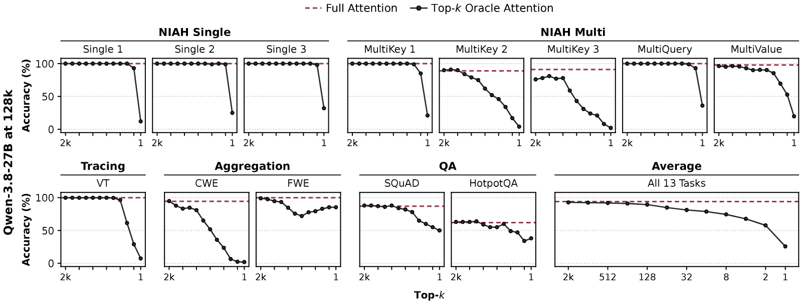
Read it carefully, because it answers two questions at once (reported). First, how many keys: with the exact top- chosen by summed attention, Qwen3.8-27B keeps 98% of its full-attention RULER score down to , which at 128k tokens is 0.8% of the keys. Single-needle retrieval survives down to . What breaks first is aggregation and multi-key retrieval: MultiKey 2 and 3 and common-word extraction (CWE) start falling almost immediately, because those tasks genuinely need many keys at once. Second, whether one shared list is enough: the oracle already sums over heads, the same restriction as LSA's index query, and it still holds at 512. So the head sum is not where the accuracy goes; the search is.
LSA ships on Qwen, eight times the oracle's comfortable floor. The slack is there because LSA's list is not the true top-; it is the top buckets by centroid, which is an approximation of it. How good an approximation is what the experiments below measure.
How LSA finds the keys
The method has two halves: build buckets once per block of keys, then search them for every query.
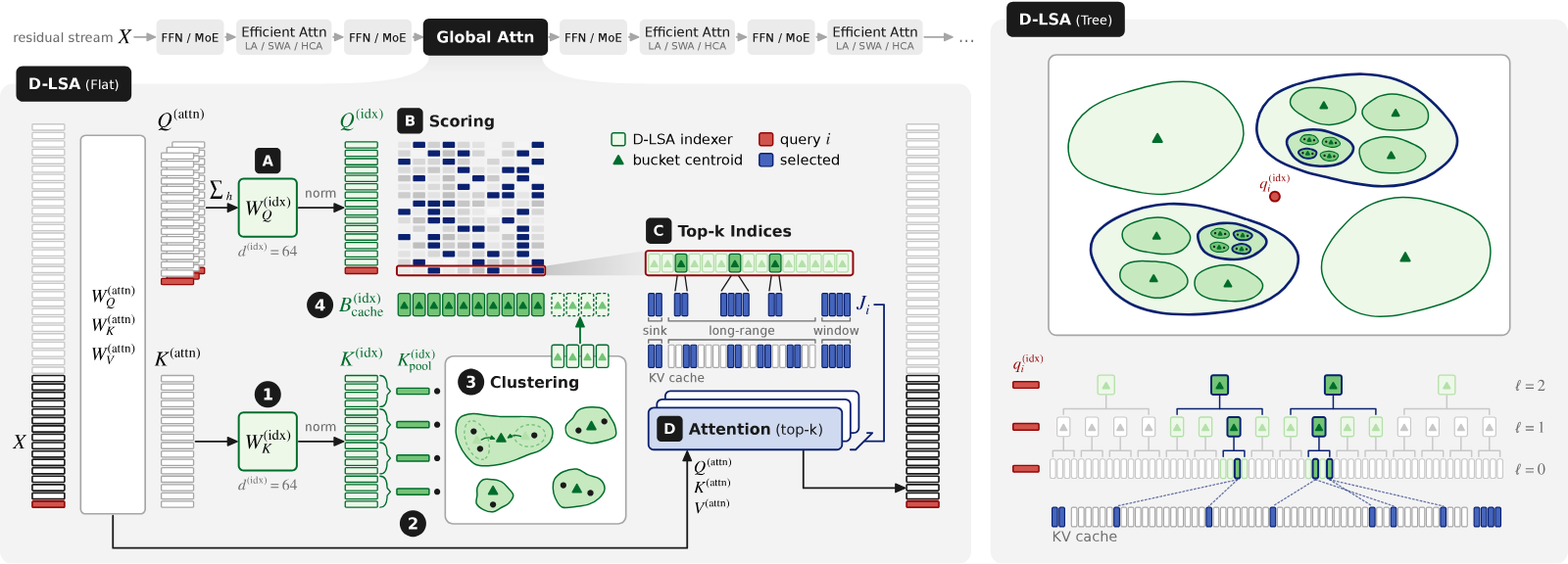
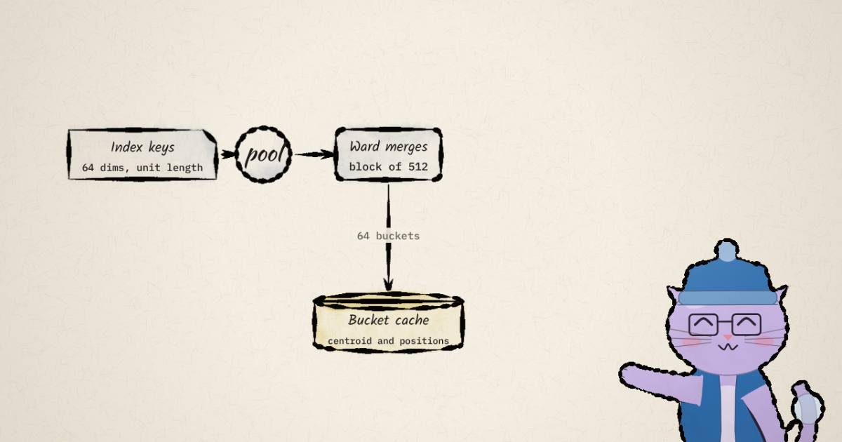
Clustering (steps 1 to 4). Each index key is projected to 64 dims and L2-normalised. Every 4 consecutive index keys are summed into one pool key. Keys are processed in cluster blocks of 512: once a block is complete, its 128 pool keys are merged bottom-up with Ward's method into 64 buckets, about 8 keys each and never more than 16. A bucket stores the normalised sum of its keys as its centroid, plus the positions of its keys. Once a block is clustered, its buckets never change.
The merge rule is worth a line of algebra, because the code's version looks nothing like the textbook one. In
src/lsa/core/ward.py the cost of merging buckets and is
For unit keys, the spread of a bucket around its unit centroid is . Merging two buckets adds their sizes, so the spread grows by exactly (reasoned, from the code). It is Ward's criterion on the sphere: merge whatever adds the least scatter. The rounds are parallel: every bucket finds its cheapest allowed partner, and every pair that is each other's cheapest merges at once.
Search (steps A to D). The index query is the sum of all query heads, projected and normalised, so one list
serves every head. It scores the centroid of every bucket in the blocks before its own, keeps the top
1,024 buckets (), and expands them best-first until it holds 4,096 long-range keys (). It also reads 4 sink keys and
a 512-key window, the window being exactly the current, not-yet-clustered block. Those are the paper's settings
and the shipped defaults in src/lsa/sglang/settings/design.py (measured).
Here is the same algorithm at a scale you can see. The index space is two-dimensional, so every unit key is a point on a circle. Ward and the search are the reference steps, ported line for line.
Switch to "topic changes every token" and leave pooling at 4. The buckets fall apart, and so does recall. A pool sums four consecutive keys before Ward ever sees them; if those four mean different things, the pool is a blend and no clustering can unblend it. With pooling off, the same keys cluster cleanly. Pooling is there for cost: Ward runs over 128 pool keys per block instead of 512, and every bucket is guaranteed at least 4 keys, which is what makes always fill the budget. Hold that thought for the experiment.
Flat and tree. Flat scores every centroid: dot products of 64 dims per query, against GLM's multiply-adds, so 128x fewer (reasoned, from the two configs). It is still linear per query. The tree variant groups 4 buckets into a node bucket, repeatedly, and beam-searches down the levels, which makes prefill . On the paper's own measurements, the tree only overtakes flat in decode from about 5M tokens with one request, and in prefill it is predicted to overtake beyond 10M (reported). Below that, flat wins.
The method, term by term
Here is the whole flat path for one layer of GLM-5.3-Flash, with shapes. is the context, the attention heads, and every index vector is 64-dimensional and unit length.
1. Index keys. Each attention key is projected and normalised:
On Qwen3.8-27B the projection reads only the part of each key that carries no rotary position, a quarter of its
dimensions being rotated (reported). GLM-5.3-Flash is an MLA model with no rotary dimensions in its keys at all,
so the repository builds its index from the 512-dimensional compressed latent every head's key comes from
(measured, src/lsa/core/index_space.py, whose docstring notes that collapsing GLM's expanded heads instead would
give 16,384 dimensions for the same selection). Either way, the index space is position-free: two keys land near each
other because of what they say, not where they sit.
2. Index query. One per token, summed over all the heads before the projection:
The sum is what makes one key list serve all 64 heads. That is a real restriction, not a detail: a head that wants something the other 63 do not cannot ask for it. The paper's appendix tests how much that costs with an oracle, in the next section.
3. Pools. Within each cluster block of 512 index keys, every 4 consecutive keys are summed: .
4. Ward. The 128 pools are merged to buckets with the cost above, cap 16 keys. A bucket stores its key sum , its alignment and its unit centroid . Per block: 64 centroids and a member table of positions, padded. Nothing is seeded and nothing is reassigned afterwards; the merges are the partition.
5. Score and pick. A query at position sees every bucket of the blocks before its own, about of them. Its score of bucket is a single dot product,
and it keeps the best. Since is the normalised mean of the bucket's keys, is proportional to the query's average score over those keys: a bucket wins when its keys agree with the query on average, not when one of them does. The code has an answer to that which the paper does not mention; it comes up below.
6. Expand. Picked buckets are read best first, their members appended until long-range keys are held, the last bucket cut short. Members that fall in the sink or the window are skipped, because the read takes those anyway. Add the 4 sinks and the 512-key window and each query reads at most keys: 2,564 below 1M tokens on GLM, 4,612 above.
7. Attend. The model's own attention runs over with its own queries, keys and values. The paper reuses existing kernels, FlashAttention-3 among them, reading as a page table.
What it costs to hold (reasoned, from those shapes, bf16 centroids and int32 members): at 10M tokens there are 1,310,720 buckets per layer, so 160 MiB of centroids and 80 MiB of member tables, about 245 MiB with the bucket sizes. The paper reports 246 MiB per layer. GLM's own indexer keeps one 128-dimensional key per 4 tokens, 2,621,440 of them, which at one byte a dimension is 320 MiB before its scales; the paper reports 331 MiB. The index keys of a closed block are not kept once it is clustered.
The tree, step by step
The tree builds levels on top of the buckets. Every 4,096 buckets form a node cluster block, and inside it the
buckets are paired by the same Ward merge with a cap of 2, then the pairs paired again, so each node bucket has
exactly 4 children (pair_into_node_buckets in hierarchy.py). Level 2 does the same over level-1 nodes, and so
on. A node's centroid is the normalised sum of every key beneath it.
The beam (beam_pick) starts at the lowest level with at most 32,768 node buckets and scores all of them. It keeps
the best 2,048, steps down to their 8,192 children plus any node buckets of that level no level above covers yet,
keeps 2,048 again, and at the bucket level picks the top from the last beam's children and the buckets not yet
under any node. Those are the shipped knobs for both models (measured,
configs/evaluation/production/*/lsa_tree_*.yaml: node_bucket_size: 4, node_cluster_block_size: 4096,
beam_width: 2048, start_nodes: 32768).
Replaying that rule (reasoned): at 1M tokens there are 131,072 buckets and 32,768 level-1 nodes, so the beam starts at level 1 and scores 32,768 + 8,192 = 40,960 vectors, against 131,072 for flat. At 10M it starts at level 3, with 20,480 nodes, and scores 20,480 + 3 x 8,192 = 45,056 against 1,310,720: 29x fewer. The count stops growing with once the start level moves up, which is the paper's . Below a few million tokens the saving is a factor of 3 or less, and the tree pays for it with several dependent rounds of top-k on the GPU instead of one, which is why, with one request, it only wins in decode from about 5M tokens (reported, Table 12: 68 µs against 86 µs at 10M, 38 against 30 at 128k; with 16 requests it already wins at 1M, 82 against 109).
Where the index space comes from
D-LSA bolts onto a trained model. It freezes everything and trains only , and a temperature per layer, minimising the forward KL divergence between what the layer attends to and what the index would pick:
is every key the query could select, outside the sink and the window. Three choices in the recipe are worth noticing (all reported). The target keeps only each query's 2,048 heaviest keys, renormalised, while spans all of , so the loss pushes probability onto the keys that matter and does not care how the long tail is ordered. The distillation scores every key directly, with no clustering in the loop, so the buckets are never trained for; they are a consequence of a good metric. And is calibrated per layer before the first step, because unit vectors give scores in , far too flat to match a peaked attention without it. Both projections start from the leading 64 principal directions of the layer's keys. The run is 352M tokens of 16k to 1M-token documents from seven domains, 48k steps of 128 queries each, learning rate , against the 2.1B tokens of DeepSeek's DSA warm-up. The model is not then fine-tuned under sparse attention.
D-LSA (Training-Free) stops at the initialisation: the principal directions serve as both projections.
N-LSA trains from scratch with no index projections at all. It clusters the attention's own keys, which needs a single KV head so that one key per token serves every query head, and scores a bucket by its best head, , instead of a sum. The gradient stops at the selection, so the next-token loss trains the projections only through the keys each query actually attended to. No teacher, no auxiliary loss, no extra parameters.
What the kernels do about the top-p
The algebra above hides the hard part of making this fast. In prefill, a chunk of 32,768 queries at 10M tokens scores a matrix of 32,768 rows by 1.3M buckets, and each row needs its top 1,024. That matrix is never written to memory (reported): it is split over many thread blocks, so no block sees a whole row, and sorting each span and merging, the FAISS way, would list 327,680 candidates per row at 10M.
The paper's answer is a threshold, after Floyd and Rivest's selection algorithm. A first pass scores a sample of buckets per row and sets at or just below the -th best sampled score, with , so that about buckets of the whole row should clear it. The bucket scan then compares each score with as it comes off the tensor cores and appends only those above it to a short list. The threshold decides how many buckets are listed, never which ones are picked: as long as at least clear it and the list has room, the true top- is inside. A row whose estimate misses falls back to scoring itself in full. A radix select over packed 64-bit keys, score bits above and inverted bucket id below, finds the cut at keys, and the list is never sorted because attention does not care about order.
The measured behaviour on real inputs (reported, GLM-5.3-Flash, 12 held-out 1M-token documents and 3 books of 10M): the list holds 1,679 buckets on average at 1M and 1,737 at 10M, against , so roughly ; it never overflows; and 5 in 100,000 prefill queries fall back at 1M, 1 in 1,000 at 10M.
Per step, for one prefill chunk at 10M tokens on an H200 (reported, Table 11): threshold estimate 2.02 ms, bucket scan 11.39 ms at 49% of the bf16 peak, candidate scoring 1.63 ms, expansion 2.37 ms, 17.41 ms in all with the CuTe DSL kernels and 39.48 ms with the portable Triton ones. Ward on the 64 cluster blocks of that chunk takes 0.043 ms. A decode step's whole selection takes 71 µs, reading the centroids at 3.58 TB/s, 75% of the HBM bandwidth: in decode the flat search is a pure memory sweep, which is why the tree catches up there first.
Precision is chosen by measurement too: bf16 centroids change about 20 of the 4,096 selected keys against fp32 and move the covered attention mass by under 0.0001; fp8 centroids changed about six times as many, so buckets stay bf16 and only the tree's node centroids drop to fp8 (reported).
What the release code does that the paper does not say
Reading src/lsa/ at commit 6291aa6 (measured), five things stand out.
- Bucket shapes.
src/lsa/core/shape.pyadds an option to score a bucket by its estimated best key rather than its mean: , with the covariance of the bucket's keys about its centroid, kept as its leading directions rounded to one sign bit per dimension, plus a floor for the rest of the trace. The defaults are and , and the Triton kernels read the packed signs. It answers the weakness of step 5 directly: a bucket with one key pointing at the query and seven pointing elsewhere has a dull centroid but a wide spread. No production config I found turns it on, and the paper does not describe it. I tried it below. - The early budget. GLM's "2,048 keys below 1M tokens, 4,096 above" in Table 2 is an
EarlyBudgetknob: a smaller top- and top- for queries before a position, so the short prefix of a long prompt is not charged the long-context budget. - One list, or one per GPU.
query_headscan beall, the design, orrank: each tensor-parallel rank sums only its own heads and selects its own list. The paper's oracle above argues the shared list is not the problem; the option exists to find out. - What the index reads. The design projects the attention's own key and query. A research option projects the attention input instead; the settings file records that it lost about 0.15 on RULER CWE at 512k tokens.
- The beam is capped by the hardware.
TOPK_LIMIT = 2048, "the most the engine's fused top-k selects", bounds both and the beam width. The shipped beam of 2,048 sits exactly on that cap, which is worth knowing before reading the beam sweep below.
There are also two research switches for building baselines on one code path: cluster_algorithm: position, which
turns buckets into runs of 8 consecutive keys (block sparse with the same machinery), and lse scores, which rank a
node by the LogSumExp of its children instead of its centroid.
Experiment 1: buckets against blocks
The repository's reference is plain PyTorch on a CPU (src/lsa/core/reference.py and ward.py), written as the
oracle its GPU kernels are tested against. This sandbox has no torch, so I ported those two files to numpy (at commit
5ebea73, a day before the tree experiment's), about 60 lines, and kept their semantics: pools of 4, blocks of 512, buckets of about 8 with a cap of 16, mutual-cheapest
Ward rounds, centroids from the normalised key sums, best-first expansion that skips the sink and the window.
The setup (measured, numpy 2.5.3, 2 threads on a shared 4-vCPU box, one seed):
- 64-dim unit index keys at 16k, 64k, 256k and 1M tokens; 64 queries at the last position.
- Every method reads 2,048 long-range keys besides a 4-key sink and a 512-key window. LSA uses top-p 512 and top-k 2,048, the GLM setting below 1M.
- Baselines: exact top-k by dot product; block sparse with blocks of 4 (scores block keys, twice LSA's index work); block sparse with blocks of 8 (scores , the same as LSA).
- Four kinds of keys. Topical: 64 topics times 8 subtopics, each 256-token document on one topic. Scattered: the same topics, but each token draws its own, so related keys sit far apart in the cache. Random: uniform on the sphere. Needle: random keys plus one near-copy of each query planted somewhere in the cache.
- Scores: the share of the exact top-64 keys found, and the attention mass captured at softmax temperature 0.1 as a share of what the exact top-2,048 captures.
What the numbers say (all measured):
- At equal index work, LSA matches or beats block sparse in every cell. Against blocks of 8, which score the same vectors, shipped LSA is ahead or tied on all 16 cells. On the needle test at 1M it finds 38 of 64 planted keys where blocks of 8 find 23.
- Against blocks of 4, shipped LSA loses. Blocks of 4 score twice as many vectors and win everywhere except topical at 64k, a tie. On scattered keys the gap is wide: at 64k, blocks of 4 find 74.2% of the top-64 and LSA 52.3%. This lines up with the paper's own design comparison only loosely, because its baselines use their own learned index spaces. It lines up closely with an independent run on real models, below.
- The pooling is the weak spot. Turn it off and LSA wins outright: on scattered keys at 64k it finds 99.4% of the top-64 against 52.3% with pools of 4 and 74.2% for blocks of 4; at 1M it is 43.8% against 14.6% and 27.4%. On the needle test it finds 62 to 64 of 64 needles up to 256k and 59 at 1M, where shipped LSA finds 38 and blocks of 4 find 54. The price is clustering: Ward over 512 keys per block instead of 128 took 12 to 26 merge rounds instead of 5 to 9, and 20 to 45 times longer in numpy (207 seconds instead of 8.7 for the 1M scattered cache).
- No structure, no free lunch. On random keys every method collapses with length, because the top-64 of 1M random keys are not near each other or near anything a summary can capture. LSA's bet is that real keys are clustered. The paper's accuracy results say that, for these two models, they are clustered enough.
The CPU timings are not GPU timings, but the shape carries over. At 1M keys, scoring every key for 64 queries took 766 ms, the blocks of 4 took 112 ms, and LSA's centroid scoring took 67 ms (measured). The whole-cache clustering was 8.0 seconds, paid once per block as the cache fills.
Why does pooling hurt so much here, when the paper's models hold their accuracy? Because the synthetic scattered
case is the worst case for it: neighbouring tokens unrelated in the index space. Real keys are locally coherent;
that is why block-sparse indexers work at all. My reading (reasoned) is that LSA's buckets bring scattered
related keys together at the bucket scale, while the 4-key pool assumes locality at the token scale. The paper's
appendix does not report a run without pooling, and the code keeps it as an option (pool_size: None).
Experiment 2: the tree against flat, and shaped buckets
The first experiment ran the flat search only. The tree is the part of LSA that makes the claim of ,
and the paper's own accuracy figures show it weaker than flat on GLM at 10M. So I ported hierarchy.py too: Ward
pairing of buckets into node buckets of 4 within node cluster blocks of 4,096, levels stacked until a level is too
small to fill a block, and the beam read with the shipped knobs, start at the lowest level of at most 32,768 nodes,
beam 2,048. I also swept the beam down to 256 to see how much margin the shipped width has, and ran the code's
unpublished bucket shapes (rank 2, ) on the flat read.
The setup (measured, same machine and numpy): a new generator, so these numbers are not comparable with the first experiment's, only with each other. Topical and scattered keys from 64 topics of 8 subtopics, each key its subtopic plus noise; random keys; and a needle set, random keys with one near-copy of each query planted at a random position. 256k, 1M and 2M tokens; 64 queries at the last position, one seed; every method reads top- 1,024 and top- 4,096, the GLM setting from 1M and the tree's throughout. The queries see a finished context, every full block covered.
What it shows (all measured):
- At the shipped beam, the tree costs less than a point of recall at 1M. The beam of 2,048 found 97.8% of the top-64 on topical keys against 97.8% for flat, 17.9% against 18.6% on scattered, 11.1% against 11.4% on random, and 39 needles of 64 against 40. Attention mass agreed to within 0.007 everywhere at 1M. It did that scoring 43,968 vectors per query instead of 131,008, 3.0x fewer. This matches the independent ROCm notebook's finding that tree and flat agree to two decimals.
- The loss grows with every level the beam descends. At 1M the beam starts at level 1 (31,744 nodes) and descends once. At 2M level 1 has 64,512 nodes, over the 32,768 limit, so it starts at level 2 and descends twice. The gap on scattered keys went from 0.7 points at 1M to 1.3 at 2M, 13.3% against 12.0%, while the scored count fell to 38,848 against 262,080, 6.7x fewer. A beam that keeps 2,048 nodes of 15,360 and then 2,048 of 8,192 compounds two cuts.
- The shipped beam has little margin. At a beam of 256 the needle count fell to 19 of 64, and scattered recall at
2M to 9.1%, against 13.3% flat. Halving the beam to 1,024 already cost 7 needles. The beam of 2,048 is also the
engine's top-k ceiling (
TOPK_LIMIT), so the design cannot widen it without a different selection kernel. A node bucket's centroid averages 32 keys at level 1 and 128 at level 2, which is exactly where a lone relevant key disappears. - Shaped buckets help where centroids fail and hurt where they work. Scoring each bucket by its estimated best key found 49 needles at 1M against 40 for plain flat, and added 3.1, 1.8 and 0.7 points of recall on scattered keys at 256k, 1M and 2M. On topical keys it lost 1.4 points at 1M and 3.7 at 2M, and 4 points of attention mass at 1M: when buckets are coherent, a spread bonus promotes loose buckets over tight good ones. It also costs three products per bucket instead of one. That might be why it is in the code and not in the paper or any shipped config; the repository does not say.
The tree's cost is the clustering. In numpy, building the levels took 274 to 416 seconds at 1M and 609 to 826 at 2M, far more than the buckets themselves (5 to 6 seconds at 1M): pairing 4,096 buckets is a 4,096-by-4,096 merge that took about 18 to 20 mutual-nearest rounds per pass. On the GPU the paper reports 0.405 ms per node block (reported, Table 11), so this is a CPU artefact, but it says where the tree's work went: from every query to the build.
My reading (reasoned): on keys like these, the tree is a near-free approximation of flat at one descent and a measurable one at two, and the paper's own result, flat ahead of tree on GLM at 10M on RULER, 66.8 against 55.8, is the same direction at three descents with real keys. If you serve one request at a time below about 5M tokens, flat is both faster per decode step and more accurate (with 16 concurrent requests the paper's tree is already faster at 1M); the tree is for the regime where flat's linear scan is the bill.
What the paper reports
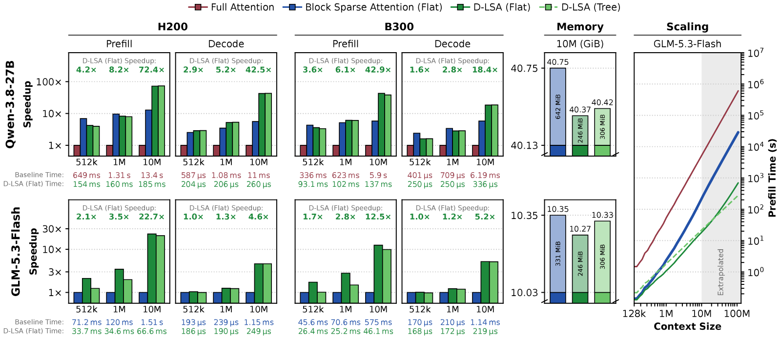
Speed (reported). On H200, one layer at 10M: 72.4x prefill and 42.5x decode over Qwen3.8-27B's full attention, 22.7x and 4.6x over GLM-5.3-Flash's sparse attention. On B300 the Qwen numbers are 42.9x and 18.4x. The index is also smaller: 246 MiB per layer at 10M against 331 MiB for GLM-5.3-Flash's indexer and 642 MiB for QSA.
The end-to-end table is where to look before getting excited. With one request at a time on H200:
| Model, parallelism | Context | Time to first token, baseline | D-LSA (Flat) | Block sparse (Flat) |
|---|---|---|---|---|
| Qwen3.8-27B, TP8 + DCP8 | 512k | 21.7 s | 1.03x | 1.61x |
| Qwen3.8-27B, TP8 + DCP8 | 1M | 65.3 s | 1.51x | 2.30x |
| Qwen3.8-27B, TP8 + DCP8 | 10M | 4582.2 s | 9.21x | 8.02x |
| GLM-5.3-Flash, CP8 | 1M | 18.1 s | 1.09x | baseline |
| GLM-5.3-Flash, CP8 | 10M | 451.5 s | 2.24x | baseline |
On Qwen, the block-sparse baseline the authors built is faster end to end than D-LSA at 512k and 1M; D-LSA wins at 10M. On B300 at 512k, D-LSA (Flat) is 0.68x on Qwen, slower than full attention (reported, Table 3). Time per output token on Qwen at 10M improves 2.87x. None of this is a criticism of the method. It is a statement of where it belongs: past 1M tokens.
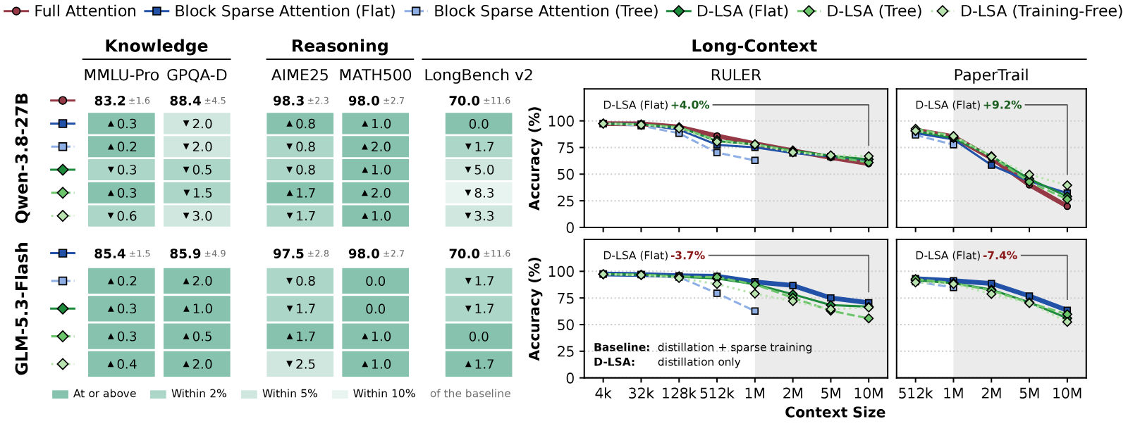
Accuracy (reported). On knowledge, reasoning and LongBench v2, D-LSA stays inside the baselines' 95% confidence
intervals. On Qwen3.8-27B, D-LSA (Flat) is within 5 points of full attention on RULER up to 1M and ahead at 10M,
63.9 against 59.9, and 29.1 against 19.8 on PaperTrail, a benchmark the authors built from recent papers with
planted fact trails. On GLM-5.3-Flash it trails the baseline by up to 8 points at 2M to 5M tokens and is within 4 at
10M. The tree variant is weaker there: 55.8 on RULER at 10M, against 66.8 for flat. Beyond 1M tokens, RULER runs 20 prompts per task,
so single-point differences there are noise. Qwen3.8-27B ships with a native context of 262,144 tokens
(measured, max_position_embeddings), so its 10M runs use YaRN at factor 40: every method is out of
distribution there, and "better than full attention" partly means "less hurt by it".
N-LSA (reported). A 0.5B hybrid, one attention layer in four, trained on 100B tokens of FineWeb-Edu at 4k and a 12B-token decay at 128k. N-LSA reaches the same validation loss as full attention, 1.085 against 1.085, where PISA, NSA and SWA end at 1.100, 1.117 and 1.154. On RULER at 128k it scores 32.2 against full attention's 34.7, with NSA at 19.2. One layer trains 1.6x faster than FlashAttention-3 at 128k, the model 1.24x faster end to end, with peak memory 6.8 GiB against 5.8 GiB per layer. It is small, flat-only and stops at 128k; the authors say so.
- license
- Apache-2.0
- branch
- main
- tests
- 290 files
- source
- 6.1 MB
- commit date
- 2026-11-04
by size of tracked source at this commit, file counts in brackets; docs, data and vendored trees excluded
local clone, 2026-11-10 at 5ebea73 — branch, commit, commitDate, fileCount, hasTests, languages, license, licenseFile, shallow, testFileCount
shallow clone: counts describe the pinned tree, not the history
The posts around it
The announcement thread from James Whittington is accurate to the paper: 98% indexing time at 10M, "up to 22.7x" faster sparse attention and 72.4x faster full attention, both per layer. A widely shared Chinese summary rounded it to "decode about 42x, first-token latency cut to about one ninth", added that these are single-layer H200 numbers and that the whole model gains less. That is a fair reading of Table 3's 9.21x.
A post from the Rapid-MLX account reports LSA running end to end on Apple Silicon: Qwen3.8-27B on an M3 Ultra at
128k, time to first token 640 s to 440 s and peak memory 40.7 GB to 28.8 GB, using LSA for prefill only and handing
decode back to dense attention because per-token routing overhead slowed decode (reported, unverified). I found
no code linked from the post. The repository I was pointed at for it, boxwrench/lsa-rocm, is something else: an
independent lab notebook on AMD ROCm, with no licence yet. It tests the training-free variant on the full-attention
layers of a 9B hybrid and a 33B dense model, and its findings (reported) match mine closely. Flat search
captures 43% to 56% of the ideal attention mass at a budget of 2,048 keys on prose and code from 32k to 917k tokens;
block sparse with blocks of 4 is as good on one model and clearly better on the other; and tree and flat agree to two
decimals. That is the training-free index, not the distilled one the paper's accuracy rests on.
What I could not run
- The GPU kernels and the served models. The CuTe DSL and Triton kernels need an H200, B300 or other CUDA GPU, and the 10M-token runs need eight of them. Nothing here checks the 72.4x.
- The repository's own Python. The reference needs torch, which this sandbox does not have; I ported it rather than installing a CUDA stack. My port matches the reference's steps but is not the reference.
- The distilled maps. They are release assets on GitHub (
d-lsa-weights-v1), which this sandbox cannot download. My experiment uses synthetic index keys, not the learned 64-dim space. - The Apple Silicon numbers. No code, no configuration, one screenshot.
- Page growth. The served tree grows its levels at page ends of 8,192 keys, so a query in the middle of a prefill sees a partly built hierarchy and scores the uncovered buckets directly. My tree experiment measures a query at the end of a finished context, with every full block covered. Mid-context queries score more vectors than mine did, never fewer.
- The kernels' threshold path. The GPU never takes an exact top-; it takes the top- of a list cut by a sampled threshold, with a fallback. The paper reports it misses for at most 1 query in 1,000, and when it does not miss it picks the same buckets as the exact rule, so my exact top- is the same selection. I did not test the sampler itself.
- Real keys. Every number in my experiments is on synthetic 64-dimensional keys. The pooling result, the tree result and the shaped-bucket result could each look different on a distilled index of a real model, in either direction. The paper's Figures 5 and 14 are the real-model evidence, and the independent ROCm notebook above is the only third-party check I found.
Where it sits against prior work
The paper's related-work table sorts sparse attention by what the indexer scores. Token-level designs, DeepSeek's DSA and MiniMax's sparse attention among them, score every key. Block-level designs score a summary per block of consecutive keys: GLM-5.3-Flash's own indexer, Qwen's QSA, NSA, MoBA, PISA and others; some add a fixed number of levels. Semantic designs cluster keys by content: ClusterKV, RetroInfer, Squeezed and Multipole Attention, LycheeCluster, IceCache. LSA is in the last group, and its claims against that group are scale (accuracy and speed at 10M tokens, where the others stop at 1M or below) and the training recipe (a distilled metric made for clustering, instead of the model's raw keys). The paper does not run any of the semantic baselines; its baselines are the two models' own attention and block-sparse indexers the authors built in the same code (reported, Table 1).
The block baseline's strongest case is in the appendix, and it is worth seeing next to my pooling result.
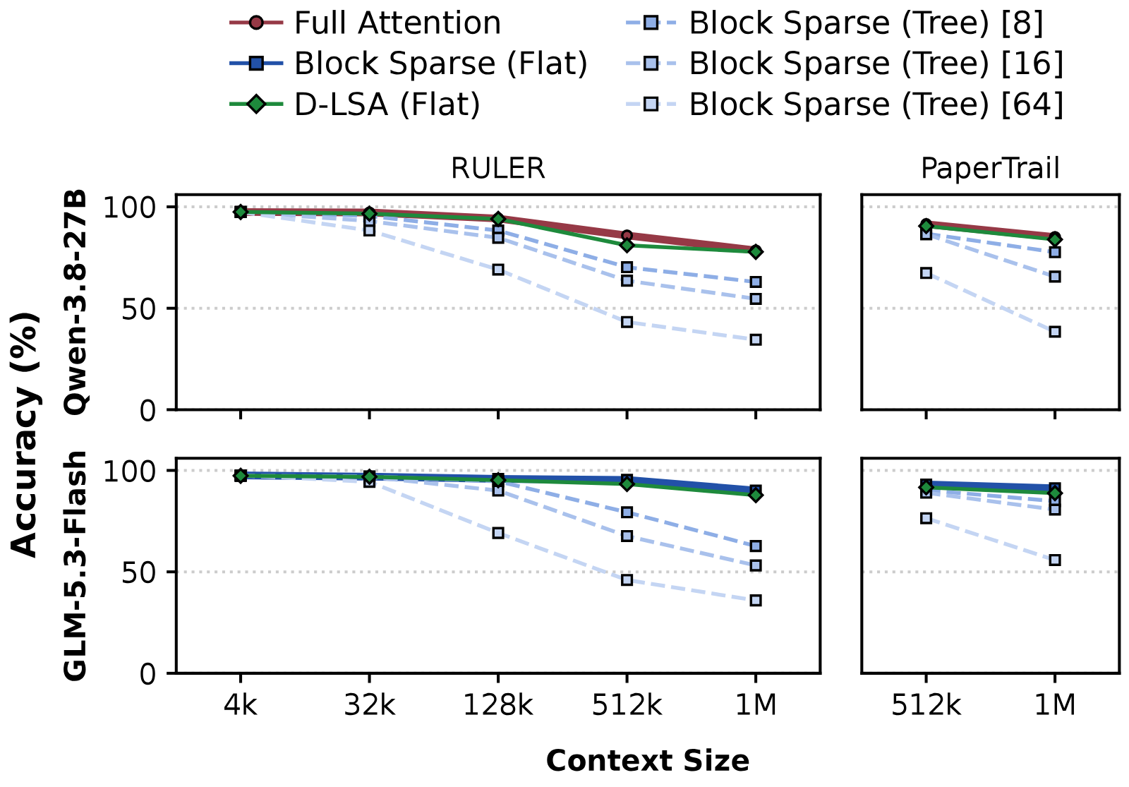
Bigger blocks fall earlier and further, on both benchmarks and both models, because one summary per block can hide a single relevant key (reported). That is the mechanism behind my pooling result, seen from the other side: a block of consecutive keys and a pool of four consecutive keys both average before anything is scored. LSA's bucket of 8 is not consecutive, which is the whole point; its pool of 4 is. Note also what the figure leaves out of its headline: the flat block-sparse baseline, which scores every block of 4, is about as accurate as D-LSA on GLM at 1M, and on Qwen it was faster end to end at that length. LSA's case rests on the contexts past 1M, where that flat scan becomes the bill.
On this site, MiniMax Sparse Attention is the scan done cheaply and per GQA group; the linear-attention roundup gives up exact recall for a fixed state; KVzip shrinks the cache itself instead of choosing within it. LSA keeps every key and exact attention over a chosen set, and spends its effort on making the choosing cost an eighth of a scan (flat) or close to a constant (tree).
What to take from it
- The cost of sparse attention at long context is the search, not the attention. Any design whose indexer touches every key, even compressed four to one with a small head, is quadratic in prefill, and at 10M tokens that is nearly all of the layer.
- LSA's speedup is real only past about 1M tokens. Below that, on the paper's own end-to-end table, a well-built block-sparse indexer is as fast or faster. If your contexts are 128k, this is not your bottleneck.
- Semantic buckets beat positional blocks at equal index cost. That held in every cell I measured. They do not beat a positional index that does twice the work, unless the pooling goes.
- The tree is cheap at one descent and not free at two. At the shipped beam it lost under a point of recall at 1M and 1.3 points at 2M on scattered keys while scoring 3x and 6.7x fewer vectors, and the beam of 2,048 sits on the engine's top-k ceiling with little margin below it.
- Check the 4-key pooling against your own keys. If neighbouring tokens are coherent in your index space, it is nearly free. If they are not, it throws away what the clustering was supposed to find.
- architecture
- Qwen3_5ForConditionalGeneration
- task
- image-text-to-text
- library
- transformers
- license
- apache-2.0
- safetensors
- 18 shards
- largest file
- 3.99 GB
- files
- 32
- downloads
- 7.1M
- likes
- 16.0K
repo last modified 2026-08-14
- architecture
- Glm5NextForConditionalGeneration
- task
- image-text-to-text
- library
- transformers
- license
- mit
- safetensors
- 62 shards
- largest file
- 5.37 GB
- files
- 73
- downloads
- 3.5M
- likes
- 2.5K
- languages
- en, zh
repo last modified 2026-09-07