2026-11-09 · 36 min · kimi · mixture-of-experts · pruning · quantization · vllm
Why read this
Notabletop 60%Confirms all 92 routers byte for byte, walks REAP's math, and prunes a real 16B relative eight ways on CPU: the shipped score loses to random.
- Checked against the source
- Interactive explanations
- Concrete numbers to act on
Quantization & compressionNeeds datacenter GPUsCustom licencePractitioner model
How this was scored
- Is it new?
- 1 of 3: An incremental tweak
- Can I trust it?
- 3 of 3: Reproduces the headline result, or shows from primary files it is wrong
- Can I run it?
- 1 of 3: API-only, gated or restrictive licence
- Will I understand it?
- 3 of 3: Mechanism carried by interactives built from real code or data
- Can I act on it?
- 2 of 3: A concrete recipe, numbers or comparison
- Will it last?
- 1 of 3: Relevant for months
- Does it affect many?
- 1 of 3: A specialist community
- Only here?
- 2 of 3: A teardown or measurement few others did
Score 66 of 100, ranked 254 of 701 rated articles. Each question is answered 0–3 by hand, and a 3 is rare. How articles are scored
On 5 November, three days after Moonshot put the Kimi K3.1 Pro weights on Hugging Face, a
repository called vllm-project/Kimi-K3.1-Pro-pruned75 appeared beside it. A post that went round the same evening
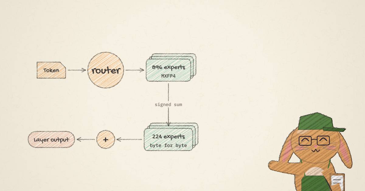
summed it up: "Original: 896 experts per MoE layer. Removed: 672 experts (75%). Remaining: 224 experts (25%)",
2.8 trillion parameters down to "~700–750B", "476 GB". Then the question everyone asks of a pruned model: "Anyone want to
try it out?"
I did not run it. It still needs four datacenter GPUs. What I could do from a sandbox with no GPU was read both checkpoints' safetensors headers by HTTP range, stream every router matrix from both repos (92 layers, about 1.5 GB in all, never stored), and check three things the card claims: what was cut, how the survivors were chosen, and what it costs to serve. Then I built a small synthetic MoE in numpy to see when the card's choice of ranking can work at all.
Every claim below is labelled measured (I computed it from the files), reported (a card or post says it) or reasoned (my arithmetic or inference on top of the measured numbers).
- architecture
- KimiK31ForConditionalGeneration
- task
- image-text-to-text
- library
- transformers
- license
- other
- safetensors
- 96 shards
- largest file
- 5.19 GB
- files
- 112
- downloads
- 286
- likes
- 20
repo last modified 2026-11-05
What the card says it is
The model card is short and unusually candid. In its own words (reported):
- "A calibration-free, expert-pruned checkpoint" that "removes 75% of the routed experts in every MoE layer".
- "Intended for vLLM serving and evaluation smoke tests on fewer GPUs, not for quality-sensitive use. Expect a large quality regression relative to the source model."
- Ranking: the "signed sum of each expert's router row,
sum(router.weight[i]), computed independently per layer". - Removed: the expert tensors, the matching rows of
gate.weightand entries ofgate.e_score_correction_bias. Experts are renumbered andnum_expertsset to 224. - Unchanged: attention, the shared experts, the dense first layer, the vision tower, and the original MXFP4 quantization of the routed experts. "Calibration data: none."
- Produced with the
MagnitudeExpertPrunerconverter in compressed-tensors, "with its default L1 scoring (weight.abs().sum(-1)) replaced by a signed sum. On this model the signed ranking scored much higher (GSM8K 43.7% vs. 14.4% for L1)."
So this is not a REAP checkpoint and does not pretend to be. The sibling it was modelled on,
vllm-project/Kimi-K3-pruned75, says why it exists: vLLM's CI needs a K3-shaped checkpoint that fits on fewer GPUs
"while accurate calibration-based pruning, such as REAP support in llm-compressor, is under development" (reported).
That framing matters for everything below. It is a test fixture with real weights, published in the open.
I checked the converter's default from the published wheel rather than the card: compressed-tensors 0.20.1 on PyPI,
entrypoints/convert/converters/magnitude_expert_pruner.py, computes scores = weight.abs().sum(dim=-1) over each
router row and keeps the max(1, num_experts - round(sparsity * num_experts)) largest (measured, read from the
source). At 896 experts and a sparsity of 0.75, that is 224.
- license
- Apache-2.0
- branch
- main
- tests
- 104 files
- source
- 1.4 MB
- commit date
- 2026-11-09
by size of tracked source at this commit, file counts in brackets; docs, data and vendored trees excluded
local clone, 2026-11-10 at 70e7167 — branch, commit, commitDate, fileCount, hasTests, languages, license, licenseFile, shallow, testFileCount
shallow clone: counts describe the pinned tree, not the history
The diff, from the headers
Both repositories ship 96 shards. I read the first eight bytes of each shard for the header length, then the JSON header itself, 192 small range requests in all (measured):
| Kimi K3.1 Pro | pruned75 | |
|---|---|---|
| tensors in the headers | 497,340 | 126,396 |
| MoE layers | 92 | 92 |
| routed experts per MoE layer | 896 | 224 |
config.json fields that differ | 1 (num_experts) | |
| parameters (Hugging Face count) | 2,780,110,363,392 | 737,611,524,480 |
| routed-expert parameters | 2,722,740,830,208 | 680,685,207,552 |
| everything else | 57,369,533,184 | 56,926,316,928 |
| tensor payload | 1,561,217,377,280 B | 475,488,771,584 B |
Each expert is three matrices, w1 and w3 of 3,072 by 3,584 and w2 of 3,584 by 3,072, so 33,030,144 parameters.
K3's experts work in a 3,584-wide latent space (routed_expert_hidden_size) behind a shared up and down projection
from the 7,168-wide residual, the "Stable LatentMoE" of the K3 article. They are stored as
MXFP4: a weight_packed U8 tensor holding two 4-bit values per byte and a weight_scale U8 tensor with one exponent
per 32 values, 17,547,264 bytes an expert (measured). Multiply out: 33,030,144 times 896 times 92 is exactly the
2,722,740,830,208 routed parameters the Hugging Face API reports for the source, and the same times 224 is exactly
the pruned figure. The API counts the packed tensors in logical 4-bit values, not bytes, which is why its "U8" line is
almost twice the bytes on disk (measured).
The rest of the diff is the router. The 672 dropped rows of gate.weight per layer, 7,168 BF16 values each, are
443,154,432 parameters across 92 layers, and the 672 dropped bias entries are the 61,824 missing F32 values. Nothing
else changed: the BF16 attention, shared experts, latent projections, norms, embedding, head and vision tower are
the same tensors at the same shapes (measured, by name and shape; I did not hash their bytes).
Both of the post's numbers hold. 737.6B is inside "~700–750B", and 475.5 GB is its "476 GB". The card's "~443 GB" is the same payload in binary units: 475,488,771,584 bytes is 442.83 GiB. The source's "~1.5 TB" is 1,561.2 GB, or 1,454.0 GiB (measured, reasoned on the unit).
One more ratio, because it decides what the next compression step should be. In the source, routed experts are 92.6% of the bytes. In the pruned checkpoint they are 76.1%. The non-expert part, 114.8 GB of BF16 and F32 in the source, was 7.4% of the bytes; at 113.9 GB it is now 23.9% (reasoned from the measured bytes). Cutting experts further now gains less than quantizing what was left alone.
Checking which experts survived
A config saying 224 does not tell you which 224. The router does. Each row of gate.weight is one expert's
fingerprint, a 7,168-vector the token's hidden state is dotted with. If the pruned router's rows are copies of
source rows, matching them recovers the selection exactly. This is the method from the
Comet 60B teardown, where it took cosine matching because the rows had been refit. Here a byte
hash is enough.
For each of the 92 MoE layers I range-requested the source gate.weight (896 by 7,168 BF16, 12.8 MB) and
e_score_correction_bias, the same two tensors from the pruned repo, hashed every row, matched them, and recomputed
both rankings in float64 (measured):
- All 20,608 pruned rows match a source row byte for byte. No row was modified or refit.
- In every layer, the kept set is exactly the top 224 by signed row sum. Not most layers: all 92.
- The order is preserved. Kept experts are renumbered in ascending source order, so expert 0 of the pruned model is the lowest-numbered survivor.
- The balance bias is carried with its expert. The pruned bias vector equals the source bias at the kept indices.
The margin at the cut is thin. Signed sums have a standard deviation of about 3.85 within a layer, and the median gap between the 224th and 225th expert is 0.0086 (measured). That matters for reproduction: a different summation order in BF16 could, in principle, swap a boundary pair. In float64 my selection and the shipped one agree in every layer.
The interesting number is the comparison. Had the converter run with its default L1 score, it would have kept a mostly different set: the two scores agree on a mean of 68.6 experts out of 224 per layer, with a range of 51 to 90 (measured). Two random picks of 224 from 896 share 56 on average. The two calibration-free rankings are only slightly better than independent of each other, and the card reports 43.7% against 14.4% on GSM8K between them. Two cheap proxies that disagree this much cannot both be good estimates of the same thing.
I also checked the one usage-derived signal the checkpoint carries. K3 routes with topk_method: noaux_tc, the
auxiliary-loss-free scheme in which each expert has a bias added to its score for selection only. During training the
bias is nudged down when an expert is overloaded and up when it is idle. If the signed row sum tracked how often an
expert is picked, it should correlate with that bias. It does not: the Spearman correlation between the two averages
0.018 across the 92 layers, and stays within ±0.2 in every layer. The 224 lowest-bias experts share 52.6 of 224 with
the signed-sum set on average, which is chance (measured). The biases are not all zero; they have a standard deviation
of 0.054 and run from −0.76 to 0.15. They are simply unrelated to the ranking.
What the checkpoint cannot tell me is how often each expert is used on real text. That needs forward passes through a 2.8T model, which is the calibration step the card deliberately skipped.
What did not get smaller
Pruning removes experts from the pool, not from the token's path. The config still says num_experts_per_token: 16,
so each token in each MoE layer still runs 16 routed experts plus the two shared ones. Counting what one text token
touches, 16 times 92 experts at 33,030,144 parameters each is 48.62B, plus every non-routed tensor except the
embedding table (one row is read) and the vision tower. That gives 104.37B active for the source, which matches
Moonshot's "104B", and 103.92B for the pruned model (reasoned from measured counts). The only active parameters that
went away are the 672 router rows per layer the scores are no longer computed against.
So per-token compute is unchanged, and so is the per-token weight traffic of a single-stream decode. What changes is how many distinct experts a batch can touch. With 64 tokens each picking 16 of 896, a uniform router would hit about 613 experts per layer per step; picking from 224, every one of them, 224 (reasoned, from 1 − (1 − 16/E)^64). A batched decode reads fewer distinct expert weights per step, which helps, but the model is not "four times faster". It is four times smaller in the one place that was large.
Memory and GPU count
Weight bytes set the floor for how many GPUs you need. The source, as shipped, is 1,561.2 GB, which is more than one 8-GPU node of anything but B300. The pruned checkpoint is 475.5 GB. The planner below takes the measured parameter counts and re-prices them at other precisions, then finds the smallest power of two GPUs whose share fits in 90% of each GPU's memory. Powers of two, because tensor parallelism has to divide both 224 experts and 96 attention heads.
As shipped, that gives (reasoned, weights only):
| GPU | Kimi K3.1 Pro | pruned75 |
|---|---|---|
| H100 80 GB | 32 (4 nodes) | 8 |
| H200 141 GB | 16 (2 nodes) | 4 |
| B200 180 GB | 16 (2 nodes) | 4 |
| B300 288 GB | 8 | 2 |
Four times fewer GPUs at every size, which is the point of a CI fixture. The card's own serving line is
--tensor-parallel-size 4 on B300, which leaves about 169 GB a GPU free after weights. That is generous on purpose:
K3's million-token window needs it. The Kimi K3 sibling's card measured what vLLM actually allocated on four GB300s:
"Model memory: 119.06 GiB per GPU" and 7,615,283 tokens of FP8 KV cache (reported). Four times 119.06 GiB is 476.24
GiB, 7.6% above its 442.50 GiB payload (reasoned), so real per-GPU shares run a little over the even split.
Two re-pricings are worth reading off the planner. Upcasting the pruned model to BF16 would make it 1,475.2 GB, about
the size of the source as shipped: MXFP4 and 75% pruning each buy roughly a factor of three. And storing the
non-expert part in FP8 instead of BF16 takes the pruned model from 475.5 GB to 418.5 GB without touching an expert
(reasoned). Whether K3's attention and latent projections survive FP8 is a question nobody has published an answer
to; the quantization config deliberately leaves self_attn, shared_experts and the latent projections out of MXFP4.
How expert pruning chooses
There are three families of answers to "which experts can go?", and they differ in what they need to see.
Router frequency. Run a calibration set through the model, count how often each expert lands in a token's top-k, drop the least used. It is the obvious baseline. It needs real forward passes, and it says nothing about how much an expert contributes when it is picked.
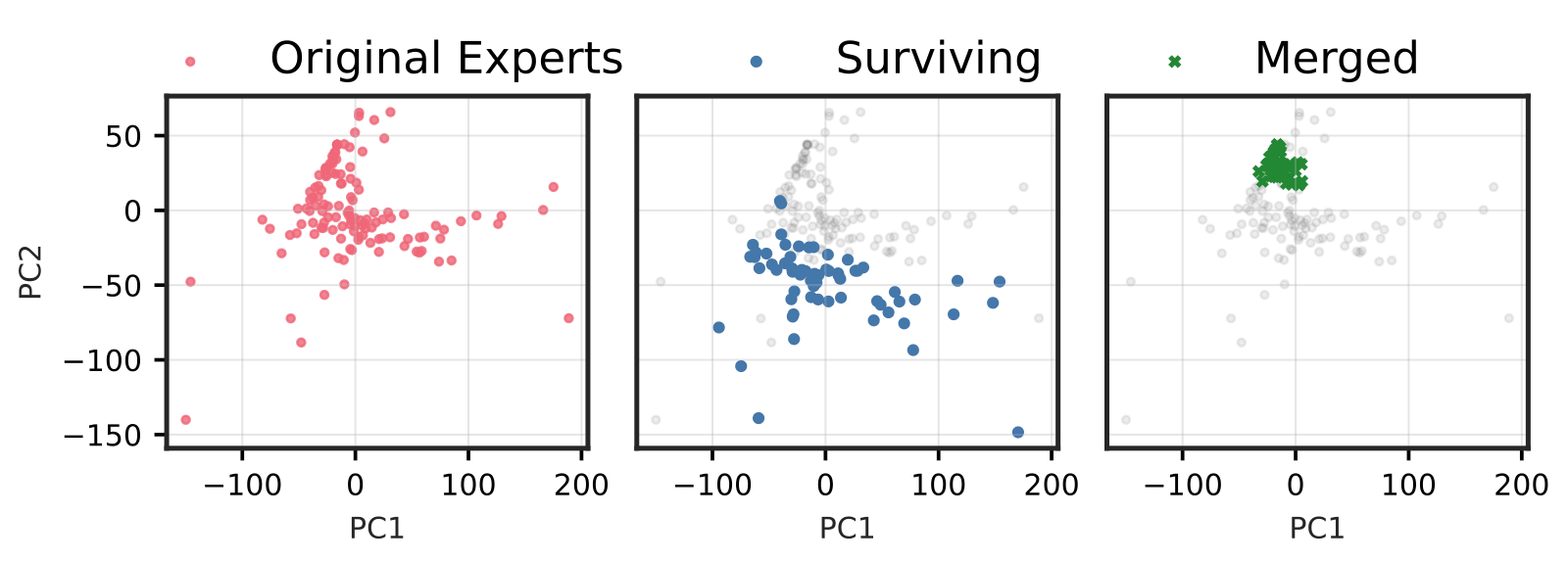
REAP. Cerebras' Router-weighted Expert Activation Pruning (arXiv 2510.13999, Lasby and colleagues) scores each expert by the average, over the calibration tokens routed to it, of its gate value times the norm of its output (reported; the Comet 60B article covers a model pruned with it). It also needs forward passes, and adds the output norm, so a rarely picked expert that matters a great deal when it is picked can survive. Runtime dynamic compression goes a step further and swaps the resident set every 256 tokens.
Weight-only scores. Look at the router rows alone. L1 magnitude is the converter's default; the signed sum is what shipped. They need no data at all, which is the only reason to use them.
The vLLM card names REAP as the thing this checkpoint stands in for, so it is worth reading what REAP actually argues, term by term, before asking how far a data-free score can get.
The layer, written out
An MoE layer with experts sends token to the set of its top-k router scores and mixes their outputs with gates that are zero outside that set and sum to one inside it (the paper's Equation 1, reported):
For Kimi K3.1 Pro the pieces have these shapes (measured from the config and headers above): is the 7,168-wide
residual, projected to a 3,584-wide latent before the experts; each is a SwiGLU block with w1 and w3 of
3,072 by 3,584 and w2 back; is 896 before pruning and 224 after; . The gate is a sigmoid
of the router logit , chosen on sigmoid plus the balance bias, then renormalised over the 16 without it.
Pruning expert removes one term. If the router simply dropped it and renormalised, the output would be the paper's Equation 2:
A real top-k router does not leave the slot empty: the next expert in line, call it , is promoted with some new gate . The paper splits the resulting error (Equation 7, reported) into a substitution error, , the output of a different function in the old one's place, and a renormalisation error that only rescales the surviving experts. The first dominates, and since a promoted expert never scores higher than the one it replaced, , it is bounded by Equation 8:
REAP minimises the part of that bound it can know in advance. Which expert gets promoted changes token to token, but is a property of the expert being removed. So the score is its average over the tokens that actually route to (Equation 9):
The two baselines it is tested against are the same sum with pieces missing. Frequency pruning keeps : it counts, and treats every pick as equally important. EAN (Jaiswal and colleagues) keeps : output norm without the gate, summed rather than averaged, so it is still dominated by how often an expert is picked. REAP divides by on purpose. A specialist that fires on 0.1% of tokens with a large, confidently gated output scores as high as a generalist with the same per-token contribution (reasoned from the definitions).
Merging is the alternative the paper argues against. Collapse experts and into one with the summed gate , and the router can no longer mix them in an input-dependent ratio . Under the paper's simplifying assumptions, the best constant merge still pays (Equation 6):
That is zero only if the router always mixes the pair in the same ratio or the two experts compute the same thing. Fine-grained MoEs, many small experts and a variable router, are where neither holds. The pruned75 checkpoint does not merge anything, so it keeps what the paper calls "independent control" over every surviving expert. What it gives up is the choice of which 224.
What the paper measured
The calibration is not small. For models up to 110B the paper packs 1,024 samples into sequences of 2,048 tokens; for larger ones it uses 12,228 samples of up to 16,384 tokens, without packing, and it prunes 25% or 50% of the experts in each layer, one shot, no fine-tuning (reported).
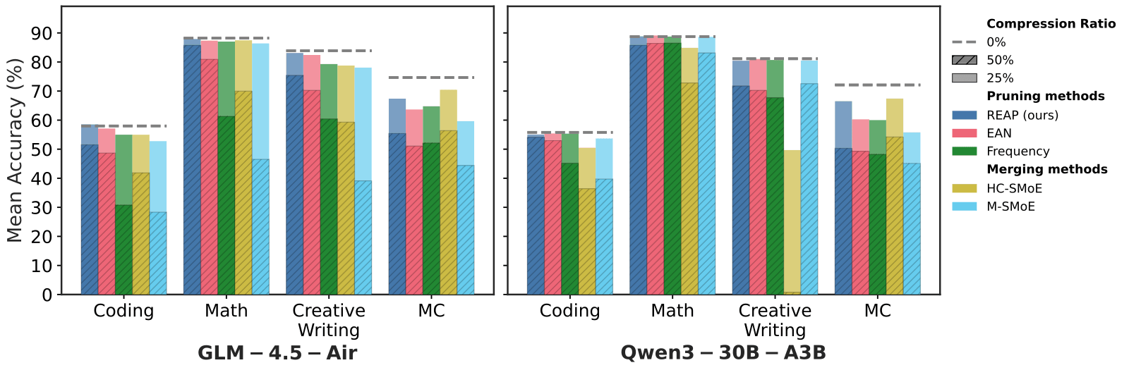
The row that matters most here is Kimi-K2, Moonshot's earlier 1T-parameter model with 384 experts a layer, pruned in its INT4 form. From the paper's Table 3 (reported):
| Kimi-K2-Instruct W4A16 | EvalPlus | LiveCodeBench | SWE-bench Verified | BFCLv3 overall | MC average |
|---|---|---|---|---|---|
| unpruned | 0.828 | 0.434 | 0.554 | 0.666 | 0.780 |
| 25%, frequency | 0.486 | 0.082 | 0.000 | 0.431 | 0.604 |
| 25%, EAN | 0.779 | 0.379 | 0.562 | 0.652 | 0.703 |
| 25%, REAP | 0.840 | 0.440 | 0.580 | 0.635 | 0.773 |
| 50%, frequency | 0.112 | 0.000 | 0.000 | 0.218 | 0.439 |
| 50%, EAN | 0.722 | 0.253 | 0.576 | 0.573 | 0.587 |
| 50%, REAP | 0.819 | 0.429 | 0.576 | 0.564 | 0.643 |
Two things in that table bear on pruned75. First, on a Kimi model the choice of score is not a detail: frequency pruning at 25% already takes SWE-bench from 55.4% to zero, while REAP at 50% keeps it at 57.6%. Second, the paper stops at 50%. Nobody has published what REAP does to a Kimi model at 75%, so "REAP would have done much better" is a reasonable expectation, not a measured fact (reasoned).
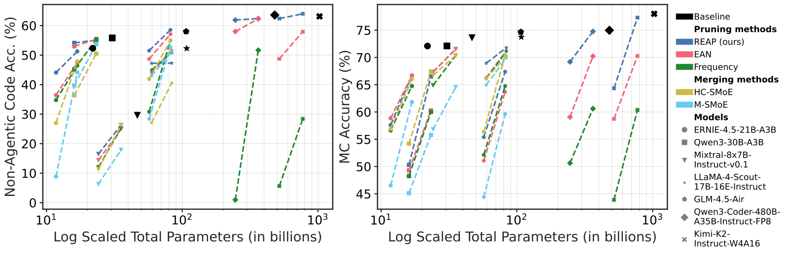
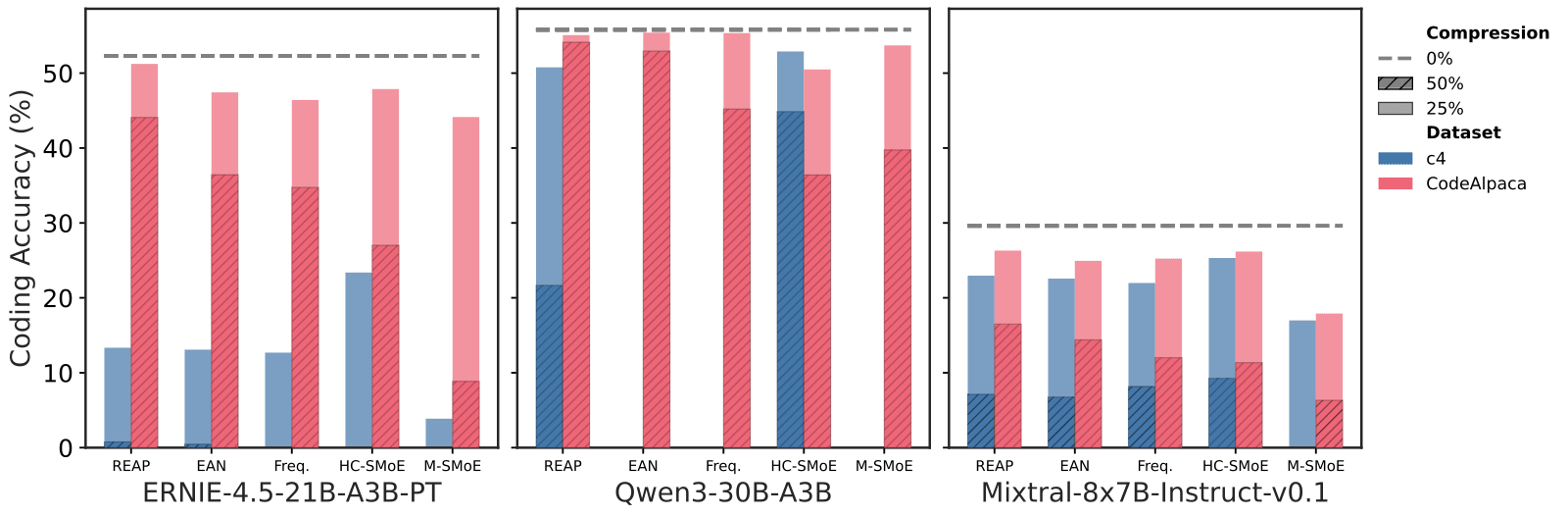
The calibration set matters as much as the score. Calibrated on C4 web text instead of code, the same methods lose most of their coding accuracy, and on Qwen3-30B several produce no usable code at all (reported, Figure A8). A calibration-free checkpoint skips this question rather than answering it.
What the released REAP code does that the paper does not say
The paper writes as the model's gate. The public repository,
CerebrasResearch/reap at commit 1970473 (17 April 2026), computes
something close to it but not always the same (measured, from src/reap/observer.py and
src/reap/pruning_metrics.py):
- The observer picks each token's experts with
torch.topk(router_logits, top_k), on the raw logits. A DeepSeek-V3-style router, which is what Kimi uses, picks on sigmoid score plus the balance bias, so the observer's is not the set of tokens the model actually sent to . - The gate is
F.softmax(router_logits, dim=1)over all experts, renormalised over the chosen top-k when the config setsnorm_topk_prob(the defaultrenormalize_router_weights=True). For a softmax router that is the real gate. For a sigmoid router the real gate is renormalised, a much flatter weighting. - The model registry covers Qwen3-MoE, Llama 4, Mixtral, DeepSeek-V2, ERNIE 4.5 and GLM-4.5. It has no
DeepseekV3ForCausalLMentry, the class Kimi-K2 and K3 load as, so the Kimi-K2 results above came from code that is not in this snapshot (reasoned from the registry).
None of that makes REAP wrong; it makes "REAP" a family of slightly different scores. I measured how much the difference matters on a real sigmoid-routed model below.
Why a signed row sum could mean anything
Why would the signed sum of a router row mean anything? The router's logit for expert on hidden state is . Write as a shared mean plus a token-specific part. Averaged over tokens, the logit is . The signed sum is , the same dot product against the all-ones vector. So the signed sum ranks experts by their expected logit exactly when the mean hidden state points along all-ones, and in proportion to how much of does (reasoned). L1 magnitude, by contrast, ranks rows by how large they are in any direction, which says little about whether the hidden states ever point their way. I cannot measure for K3 without running it. I can measure it for a smaller model built the same way, which is what the Moonlight section below does.
A toy: when can a weight-only score stand in for frequency?
To see the mechanism, I built one MoE layer in numpy routed the way K3's is: sigmoid scores, the top 4 of 64 experts chosen on score plus a balance bias, gates renormalized without the bias, each expert a small ReLU MLP. Hidden states are a shared offset plus Gaussian noise. I pruned to 8, 16, 32 or 48 experts by four scores, measured on 6,000 calibration tokens where a score needs them, and compared the pruned layer's output with the full layer's on 6,000 held-out tokens. The error is squared error over the squared size of the full output, so 1.0 is as bad as deleting the routed output entirely. Eight seeds, numpy 2.5.3, two threads, 45 seconds (measured). The core:
# toy3.py (core). W: router (E, d); b: balance bias; ids: experts kept
def route(X, ids):
    s = 1 / (1 + np.exp(-(X @ W[ids].T)))                # sigmoid scores
    top = np.argsort(-(s + b[ids]), 1)[:, :k]             # bias picks, does not weigh
    g = np.take_along_axis(s, top, 1)
    return np.asarray(ids)[top], g / g.sum(1, keepdims=True)

if balanced:                                              # aux-loss-free balancing
    for _ in range(300):
        e, _ = route(Xc, np.arange(E))
        load = np.bincount(e.ravel(), minlength=E)
        b -= 0.002 * np.sign(load - load.mean())

scores = {"frequency": np.bincount(ec.ravel(), minlength=E),
          "signed": W.sum(1), "l1": np.abs(W).sum(1), "random": rng.random(E)}
Keeping 16 of 64, the same 25% as the real checkpoint (measured, toy):
| hidden-state offset | load | frequency | signed sum | L1 | random |
|---|---|---|---|---|---|
| along all-ones | skewed | 0.737 | 0.753 | 1.306 | 1.435 |
| random direction | skewed | 0.711 | 1.445 | 1.350 | 1.437 |
| along all-ones | balanced | 1.454 | 1.443 | 1.460 | 1.473 |
| random direction | balanced | 1.456 | 1.461 | 1.469 | 1.472 |
Three things fall out of it.
- The signed sum is a frequency estimate in disguise, when the geometry lines up. With the offset along all-ones, it keeps 14.5 of the 16 experts frequency would keep, and its error is within 0.02 of frequency's. Move the offset to a random direction and it keeps 4.1 of 16, which is what random keeps, with the same error as random.
- L1 does not track usage in either case. It is a little better than random on average, nowhere near frequency.
- Balancing removes most of what any ranking can find. Without the bias, the 16 most-used experts handle 60.6% of routing decisions; with it, 25.7%, barely above an even quarter. Then frequency, signed sum, L1 and random all land between 1.443 and 1.473. When every expert does a share of the work, dropping three quarters of them drops three quarters of the work, whichever three quarters you pick.
Above 1.0 is not a bug. When a token's chosen experts are gone, the renormalized gates put full weight on whichever survivors it scores highest, which can be further from the right answer than nothing.
The toy's experts are independent random networks with similar output sizes, so none is a specialist and none is
redundant with another. That leaves out exactly what REAP's score is built to see, an expert that is rarely picked but
large when it is, so I left REAP out of the toy. An earlier version of this article also read the balanced rows as a
forecast for K3: K3 is trained with noaux_tc balancing, so its load "should be" flat. The next section measured that
on a real model of the same design, and it is not.
The same question on real weights: Moonlight
The toy settles what a signed row sum can mean. It cannot say whether a real model's hidden states lean along all-ones,
whether a balance-biased router leaves any skew to find, or what each score costs once the damage compounds through
the layers. Those need a real MoE with K3's routing. The smallest public one I know is Moonshot's own
Moonlight-16B-A3B: the DeepSeek-V3 architecture that Kimi K2
and K3 inherit, with scoring_func: sigmoid, topk_method: noaux_tc and an e_score_correction_bias in every MoE
layer, 64 routed experts and two shared ones, the top 6 per token, routed_scaling_factor 2.446, 27 layers of which
the first is dense (measured, from its config.json). Each expert is a SwiGLU of 2,048 to 1,408 and back, 8,650,752
parameters.
- architecture
- DeepseekV3ForCausalLM
- task
- text-generation
- library
- transformers
- license
- mit
- safetensors
- 27 shards
- largest file
- 1.84 GB
- files
- 45
- downloads
- 16.3K
- likes
- 118
repo last modified 2026-01-30
How I ran a 16B model on two CPU threads
The checkpoint is 27 shards, one per layer. The script streams a layer's tensors by HTTP range into memory, runs every
token through it, drops it and fetches the next, so the 32 GB of BF16 weights pass through about 3 GB of RAM and never
touch the disk (measured, peak RSS 2,993 MB during the layers, 4,024 MB while scoring the output head). The attention,
norms and rotary embedding are the stock DeepseekV3Attention and friends from transformers 5.20.2 with PyTorch
2.14.1, loaded with Moonlight's weights; the repository's own modeling_deepseek.py and tokenizer are custom code I
did not execute. I re-implemented the two pieces that mattered instead: byte-level BPE over the published
tiktoken.model ranks with the tokenizer's split pattern, and the MoE layer itself, so that each pruned variant could
route over its own surviving experts:
# prune_moonlight.py (core). Wr: router (64, 2048); bias: e_score_correction_bias; keep: surviving ids
def route(x, keep):
    s = torch.sigmoid(x @ Wr[keep].T)                     # gate scores
    idx = torch.topk(s + bias[keep], 6, dim=-1).indices   # chosen with the bias...
    g = s.gather(-1, idx)                                 # ...weighted without it
    g = g / (g.sum(-1, keepdim=True) + 1e-20) * 2.446     # renormalise, routed_scaling_factor
    return keep[idx], g
The text is small but real. Calibration: two 512-token sequences of Pride and Prejudice from Project Gutenberg and
two of Python's standard library (json/decoder.py, argparse.py), 2,048 tokens. Held out: two sequences from the
WikiText-2 test split and two from textwrap.py and heapq.py, another 2,048. Every hidden state in the calibration
pass and 17 held-out streams (the full model plus eight scores at two keep counts) is carried layer to layer together,
so each layer's weights are fetched once. The full run took 2,630 seconds (measured).
The sanity check is the unpruned model's perplexity: 8.29 on the WikiText-2 sequences and 4.31 on the Python (measured). A broken rotary embedding or a wrong expert order gives numbers in the hundreds; these are in the range a healthy 16B model scores on encyclopaedia text in 512-token windows (reasoned).
Eight scores, each computed per layer from the full model's own calibration pass:
- frequency: how often each expert is in a token's top 6;
- REAP: Equation 9 with the model's real gate, sigmoid renormalised, over the tokens the model really sent there;
- REAP, code's gate: the released observer's version, top 6 on raw logits and a softmax gate;
- w · mean input: the router row dotted with the mean router input, the expected-logit score from the theory above, which needs one 2,048-wide vector of data rather than any expert outputs;
- balance bias: experts with the lowest
e_score_correction_bias, the ones training pushed down for being busy; - signed sum and row L1: the two data-free scores from the card;
- random, seeded per layer.
Result 1: the signed sum does not see usage, because the hidden states do not lean along all-ones
The theory says the signed sum is the expected router logit when the mean input points along all-ones. On Moonlight, the cosine between the mean router input and the all-ones vector is 0.011 averaged over the 26 MoE layers, and never above 0.040 in magnitude (measured). The mean input is, for this purpose, orthogonal to all-ones. The signed sum and the expected logit are then unrelated, a correlation of −0.075 across experts (measured), and the signed sum's rank correlation with how often experts are actually picked is −0.118 on average, slightly backwards, never above 0.003 in any layer (measured).
The expected logit itself, , is a good proxy: a mean rank correlation of 0.748 with real frequency and 11.2 of the 16 most-used experts recovered per layer, against 3.7 for random (measured). So the mechanism in the toy is right, a data-light score can see usage, and the vector it needs is the real mean, not all-ones. Computing takes one forward pass on any text. The card's own description, "calibration-free", is the one property it buys by skipping that pass.
Two more readings from the same pass (measured):
- The load is not flat. The 16 most-used experts of 64 take 63.8% of routing decisions on average, between 54.9% and 72.7% by layer, where an even split gives 25%. A balance bias evens out load over training batches; on any one text the router still prefers some experts strongly. So the toy's balanced rows were the wrong model of K3, and there is more for a good score to find than this article first said.
- The bias does not rank experts the intuitive way. Taking "lowest bias = was busiest in training" as a score gives a rank correlation of −0.253 with frequency: on this text the experts the bias favours are the ones being used, which is the bias doing its job inside the selection rather than recording history.
Result 2: what each score costs, layer by layer
For the layer-local cost, each pruned variant routes the full model's own inputs to its surviving experts, and the error is the squared distance from the full layer's routed output, relative to that output's size. Averaged over the 26 MoE layers, using each token's own relative error and taking the median token (measured):
| keep | frequency | REAP | REAP, code's gate | w · mean | bias | signed sum | L1 | random |
|---|---|---|---|---|---|---|---|---|
| 32 of 64 | 0.235 | 0.201 | 0.202 | 0.287 | 0.472 | 0.758 | 0.666 | 0.705 |
| 16 of 64 | 0.966 | 0.963 | 0.872 | 0.869 | 1.137 | 1.201 | 1.249 | 1.198 |
At half, the data-driven scores leave an error about a fifth the size of the routed signal; the signed sum leaves three quarters, the same as random. At a quarter, every score is near or past 1.0, which means the typical token's routed output is about as wrong as if it had been deleted. That is the regime pruned75 lives in.
The "all tokens" view in the chart turned up something I did not expect. In layers 3 and 6, 97% and 96% of the routed output's squared size on the held-out text sits at position 0, the first token of each sequence (measured). In layer 3 one expert, number 6, is picked 18 times in 12,288 routing decisions on the calibration set, 56th of 64 by frequency, and its REAP score is 14.96 against 0.58 for the next highest. Frequency pruning removes it at both keep counts and the layer's all-token error goes to 0.98; REAP keeps it and the error is 0.014 at half (measured). That is REAP's argument in one expert: a rarely chosen expert that carries a very large output when chosen. The likely job, writing the huge first-position activation that later attention layers use as a sink, is my inference from where the energy sits, not something I traced (reasoned).
Result 3: the whole model, every layer pruned at once
Per-layer errors compound. Pruning all 26 MoE layers by the same score and running the held-out text end to end gives these perplexities, 1,022 scored tokens per text (measured):
| keep | score | WikiText-2 | Python |
|---|---|---|---|
| 64 of 64 | unpruned | 8.29 | 4.31 |
| 32 of 64 | REAP, code's gate | 19.12 | 6.06 |
| REAP | 22.35 | 6.51 | |
| w · mean input | 25.30 | 7.26 | |
| frequency | 27.29 | 6.45 | |
| balance bias | 41.21 | 21.39 | |
| row L1 | 41.50 | 22.18 | |
| random | 58.75 | 44.53 | |
| signed sum | 879.93 | 378.91 | |
| 16 of 64 | REAP, code's gate | 63.18 | 16.00 |
| row L1 | 129.33 | 160.09 | |
| REAP | 141.77 | 25.61 | |
| balance bias | 259.42 | 241.41 | |
| w · mean input | 327.28 | 28.24 | |
| signed sum | 681.75 | 2,867.56 | |
| frequency | 1,701.76 | 164.01 | |
| random | 2,050.36 | 1,963.73 |
What I take from it (reasoned, from the tables):
- At 50%, calibration buys almost everything. Frequency and both REAP variants keep Python perplexity between 6.06 and 6.51, against 4.31 unpruned; every data-free score is at 21.39 or worse. REAP's two variants lead on prose too.
- On Moonlight the signed sum is worse than random, 880 against 59 on prose at half. Whatever made it beat L1 on K3.1 Pro's GSM8K, it is not a property of the DeepSeek-V3 design in general.
- At 75% nothing is safe. The best variant leaves prose perplexity 7.6 times the original, and frequency, which was competitive at half, collapses to 1,702 once it starts removing specialists like layer 3's expert 6. That is the same shape as Kimi-K2's frequency rows in the REAP paper.
- The two REAP variants disagree more than the gate formula suggests. Taking the top 6 with or without the bias picks the same set for only 31% of calibration tokens, and the two scores share 27.0 of 32 kept experts and 11.7 of 16 (measured). The code's version did better here at 75%, 63 against 142 on prose; with one calibration set of 2,048 tokens and one seed, I would not call that a ranking of the two.
Moonlight is not K3.1 Pro. It has 64 experts where K3 has 896, top 6 where K3 has 16, no latent projection, and a different training run, so none of these numbers transfers. What transfers is the shape: on a real model of this design the mean hidden state does not point along all-ones, the load is skewed enough for a usage-aware score to matter, and at a 75% cut the choice of score is the difference between a damaged model and a broken one.
The quality numbers
There is one, and it needs care:
| checkpoint | GSM8K 5-shot | harness | source |
|---|---|---|---|
| Kimi K3 | 95.53% | vLLM gsm8k_eval.py, 256 tokens | K3 sibling card (reported) |
| Kimi K3, pruned 50% | 68.23% | same | K3 sibling card (reported) |
| Kimi K3, pruned 75% | 34.42% | same | K3 sibling card (reported) |
| Kimi K3.1 Pro, pruned 75%, signed sum | 43.67% ± 1.37 | lm_eval flexible-extract | this card (reported) |
| Kimi K3.1 Pro, pruned 75%, L1 | 14.4% | not stated | this card (reported) |
The K3 rows are one controlled comparison: same 1,319 questions, same prompts, same hardware, same vLLM checkout, and they show a 61.11-point drop at 75%. The K3.1 Pro rows use a different harness and give no unpruned K3.1 Pro baseline at all, so 43.67% cannot be read as "K3.1 Pro loses about 50 points" except by borrowing a baseline from another model and another harness. Strict-match is 43.06%, so answer extraction is not the gap (reported). There are no coding, agentic, long-context or vision numbers, and a model that gets fewer than half of grade-school maths word problems right is unlikely to be strong on any of them (reasoned).
The card says what to expect: "Expect a large quality regression". It is right.
What I ran, and what I did not
Ran (measured):
- 192 header reads by HTTP range across both repos' 96 shards, and a full tensor-by-tensor tally.
- 368 range requests for every
gate.weightande_score_correction_biasin 92 layers of both repos, about 1.5 GB streamed into memory and reduced to per-row statistics and hashes; nothing was stored. - The signed, L1 and bias rankings in float64, and the row-hash match, for every layer.
- The toy,
toy3.py, at 64 experts, four keep counts, four conditions and eight seeds. prune_moonlight.py: Moonlight-16B-A3B streamed layer by layer, eight scores, two keep counts, 26 MoE layers, 2,048 calibration and 2,048 held-out tokens, transformers 5.20.2 and PyTorch 2.14.1 on two CPU threads, 2,630 seconds.- A read of the REAP repository at commit
1970473: the observer, the saliency accumulator and the model registry.
Read but did not run: the card's conversion script and MagnitudeExpertPruner itself, and the REAP code. The
conversion reads 1.5 TB; my numpy ranking reproduces its output in every layer, which is the part that can be checked.
For REAP I re-implemented both its published score and its code's variant rather than running the repository.
Did not run: Kimi K3.1 Pro or the pruned checkpoint. No GSM8K of my own, no tokens per second, and no measurement of K3's own mean hidden state, so the Moonlight finding that it is orthogonal to all-ones is evidence about the design, not about K3.
Limits, and where this sits
The Moonlight experiment is small in three ways that matter. The calibration set is 2,048 tokens where the REAP paper uses about two million for a model this size, and one seed; scores that depend on rare experts, REAP above all, are the ones most sensitive to that. The held-out sets are 1,022 tokens each, enough to separate 19 from 880 but not 19 from 22. And perplexity on text the model has probably seen is a weak proxy for the generative tasks where the paper shows the methods diverge most; I have no coding or maths scores for the pruned variants.
Two things here I could not explain. The signed sum beat L1 by three to one on K3.1 Pro's GSM8K, per the card, and lost to L1 by twenty to one on Moonlight's prose at half. Either K3's geometry differs from Moonlight's in a way that favours it, or a 1,319-question benchmark on one checkpoint each is a noisier comparison than it looks. And the REAP variant with the "wrong" gate did better at 75% than the one matching the model; that could be the softmax gate's sharper weighting suiting this model, or noise from one small calibration set.
On the site, the Comet 60B teardown looks at a model compressed with REAP-style pruning, and runtime dynamic compression at swapping the resident expert set while decoding. Mixture of experts from scratch covers the routing that all of this assumes, and the Kimi K3 article the architecture being cut.
The take
Kimi-K3.1-Pro-pruned75 is exactly what its card says. The 224 survivors in every layer are the top 224 by signed
router-row sum, copied byte for byte with their balance biases, and nothing else in the 2.8T model was touched. The
parameter count falls to 737.6B and the payload to 475.5 GB, which takes the weights from eight B300s to two, while
each token still runs the same 104B parameters.
The choice of score is the part to take away. Two data-free rankings of the same router rows agree on about 69 of 224 experts, barely above chance, and one does three times as well as the other on the only benchmark measured. The toy shows why that is possible: a signed row sum is the expected router logit when the hidden states lean along all-ones, and noise otherwise. On Moonlight, the closest model of the same design I could run, they do not lean that way at all, the signed sum is worse than random, and one forward pass to get the real mean input would have turned the same arithmetic into a score that tracks usage with a 0.75 rank correlation. At 75% even the best calibrated score leaves a model 7.6 times as perplexed, and REAP's own authors stopped at 50%. That is why the vLLM team calls this a smoke test and is building calibration-based REAP for the real thing. Use it to test your serving stack on four GPUs. Do not use it to judge Kimi K3.1 Pro.