FOR-species20K at 85%: a tree's point cloud as seven pictures, and the source shortcut under the score
mdjsonmcp2026-10-19 · 18 min · lidar · point-cloud · 3d · datasets · benchmarks · computer-vision · classification · on-device
A 1:45 narrated explainer, drawn in code. Every number and picture in it is this article's own; the sources are below.
› transcript
Hi, I'm Oakum! Here is how a laser scan of one tree becomes seven pictures an image network can read. Stop treating the tree as points. Render it into seven flat images holding depth, point count and height, and read those with image networks. The renderer, step by step. Centre the cloud, lowest point at ground level. Pick seven views: four sides, top, bottom, and a slice of the trunk. Project each view straight on, scale the tree to fill the frame, and drop every point into a pixel. Each pixel holds three numbers, not colours: nearest depth, point count, and height. The seven renders split into three groups: sides, top and bottom, and the trunk. Each group gets its own pretrained image network. Side features are max pooled, so no side comes first. Every tree fills the frame, so its real height is added back as one number. A small head maps it all to thirty three species. On the hidden test, the best point network scored seventy five point six, the best earlier picture method seventy nine point five. This one scores eighty five, first on the leaderboard. But each forest came from one team and one scanner. On the usual random split, these trees score ninety four point eight percent. Hold out each tree's own source for its species, and the same trees fall to sixty point two. Part of the score was the scanner. Seven pictures make a strong classifier. But test it on your own forest first. Seven renders, three networks plus height, and a big drop on unseen sources. Every source is in the full article. I'm Oakum. Bye!
Why read this
Hightop 30%Traces how a LiDAR tree becomes CNN input, checks 85% against the live leaderboard, and recomputes the 95-to-60 cross-source drop from released files.
- Original analysis
- Runs on a consumer GPU
- A lasting reference
3D & spatialGPL-3.0-or-laterPractitioner paper
How this was scored
- Is it new?
- 2 of 3: A real new idea, method or capability
- Can I trust it?
- 2 of 3: Measures key facts from files, code or configs
- Can I run it?
- 2 of 3: Open code or weights with real limits
- Will I understand it?
- 2 of 3: Mechanism from first principles with figures
- Can I act on it?
- 2 of 3: A concrete recipe, numbers or comparison
- Will it last?
- 2 of 3: A reference for a year or more
- Does it affect many?
- 1 of 3: A specialist community
- Only here?
- 2 of 3: A teardown or measurement few others did
Score 68 of 100, ranked 165 of 577 rated articles. Each question is answered 0–3 by hand, and a 3 is rare. How articles are scored
A Japanese account that summarises papers posted this with a short clip. My translation:
LiDAR × ConvNeXtV2: an AI that classifies tree species from 3D scans of trees. Trained on 17,707 trees from 3 kinds of LiDAR and 25 datasets. Classifies 33 species, first on the benchmark at 85.0% accuracy. A web app and an offline Android app are also released. Research from Purdue University, accepted at WACV 2027. Sources in the replies.
The reply links the project page for "Three LiDARs, Twenty-Five Datasets: Cross-Source Generalization in Tree-Species Recognition" by Jae Joong Lee and Bedrich Benes. The subtitle is the part the post leaves out. The paper is mostly about why a leaderboard score on this benchmark overstates how well any model recognises a species, and the first-place model is the instrument it uses to show that.
There is no preprint yet; the page says "arXiv soon". Everything here comes from the code repository (commit 39937451, 16 October 2026), its docs, its released predictions and weights, the dataset's Zenodo record, the benchmark paper by Puliti et al., and the live Codabench leaderboard. What I did:
- read the renderer, model, loss and evaluation code;
- recomputed the public-set, per-species and cross-source numbers from the released out-of-fold predictions, with my own scripts;
- pulled the live leaderboard from Codabench's API on 19 October;
- ran one fold of the 256 px model on CPU on the repo's four example scans.
Every number below is labelled measured (I computed it from a file or a run), reported (the authors' or the benchmark's figure, not re-run), or reasoned (my arithmetic on the other two).
- license
- GPL-3.0
- branch
- main
- tests
- 49 files
- source
- 432.2 kB
- commit date
- 2026-10-16
by size of tracked source at this commit, file counts in brackets; docs, data and vendored trees excluded
local clone, 2026-10-19 at 3993745 — branch, commit, commitDate, fileCount, hasTests, languages, license, licenseFile, shallow, testFileCount
shallow clone: counts describe the pinned tree, not the history
The benchmark: FOR-species20K
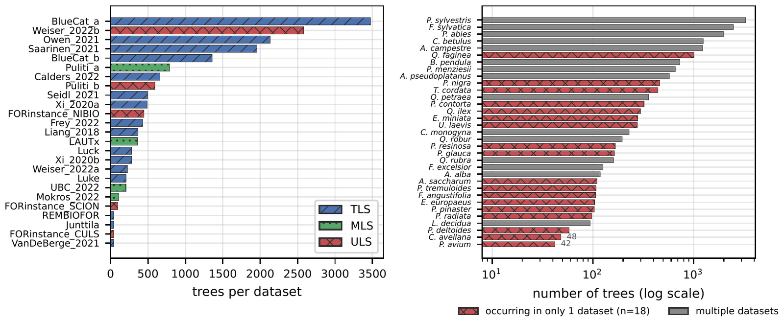
FOR-species20K (Puliti et al., Methods in Ecology and Evolution, 2025) is a set of single-tree point clouds: each file is one segmented tree, in metres, Z up, labelled with its species. The trees come from 25 source datasets, each recorded by one team in its own forest with one kind of scanner: TLS (terrestrial, a tripod on the ground), MLS (mobile, carried or driven through the stand) or ULS (a drone above the canopy).
From the metadata CSV in the repo (measured): the public labelled set has 17,707 trees of 33 species from 25 source datasets. TLS contributes 16 datasets and 12,485 trees, MLS 4 datasets and 1,464 trees, ULS 5 datasets and 3,758 trees. The classes are long-tailed: Pinus sylvestris has 3,296 trees, Prunus avium 42. And 18 of the 33 species occur in exactly one source dataset, while 6 of the 25 datasets contain a single species. That last pair of facts is what the paper is about.
A hidden test set of 2,255 trees is scored on Codabench: you upload a CSV of predictions and get overall accuracy (OA), precision, recall and F1 (reported). The test has a similar number of trees per species, so its OA behaves like the macro average of per-class accuracy, a much harsher metric than OA on the long-tailed public set, where Pinus sylvestris alone is 19% of the trees (reasoned: 3,296 of 17,707). The repo makes the same point: compare the hidden-test 85.0% with public-set macro-F1 (0.860), not public-set OA (0.899).
From points to pictures
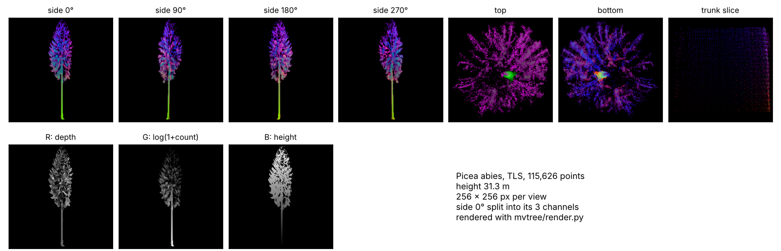
A tree scan is an unordered set of tens of thousands of XYZ points (the four example scans hold 53,839 to 150,574). A 2D CNN wants a fixed-size image. The bridge, which the authors credit to DetailView (Frey and Schindler, the previous best here), is a fixed set of orthographic renders. From mvtree/render.py:
-
Normalise. Subtract the median X and Y, and shift Z so the lowest point is at 0.
-
Pick seven views. Four sides at azimuth 0°, 90°, 180° and 270°, one along the vertical axis each way ("top" and "bottom"), and a trunk slice: the side projection of only the points between 1.0 and 1.5 m above the ground (20% to 40% of the height for trees under 5 m).
-
Project orthographically. Rotate into (image right, image up, depth), fit the larger extent into the frame with a 2% margin, and bin each point into a pixel. A 30 m spruce and a 6 m hawthorn both fill the frame.
-
Fill three channels per pixel. They are not colours:
- R: the depth of the front-most point in that pixel;
- G: , where is the number of points that landed in the pixel;
- B: the absolute height (Z) of that front-most point.
Each channel is min-max normalised to 0-255 over the occupied pixels of that view. Empty pixels stay black.
Renders are 256 or 512 px square. A side view is a silhouette with a crude depth map; the density channel carries branch structure and foliage clumping, because it counts every point, not only the front one.
One quirk: the "top" view looks along +Z and keeps the point with the smallest depth per pixel, so its depth and height channels describe the lowest surface in each column, and "bottom" the highest. It does not matter to the model, since training and inference share the code and tests/test_render.py pins it byte for byte to the loop that made the training renders.
The widget below re-implements the same rules on a synthetic tree, so you can see what the network gets as you change the render size and the scanner. The tree and the scanner sampling are made up; the projection, the channel definitions and the per-view min-max normalisation follow the code.
The scanner buttons show the problem before any network is involved. A ground scanner sees a dense stem and a thinning top; a drone sees the crown top and little stem. The species is unchanged, but the side views lose their stem and the density channel moves upward. Real scanners also differ in noise and point spacing. A classifier that sees thousands of trees per source can learn those signatures as easily as needles from leaves.
The network: three ConvNeXtV2 backbones and a height
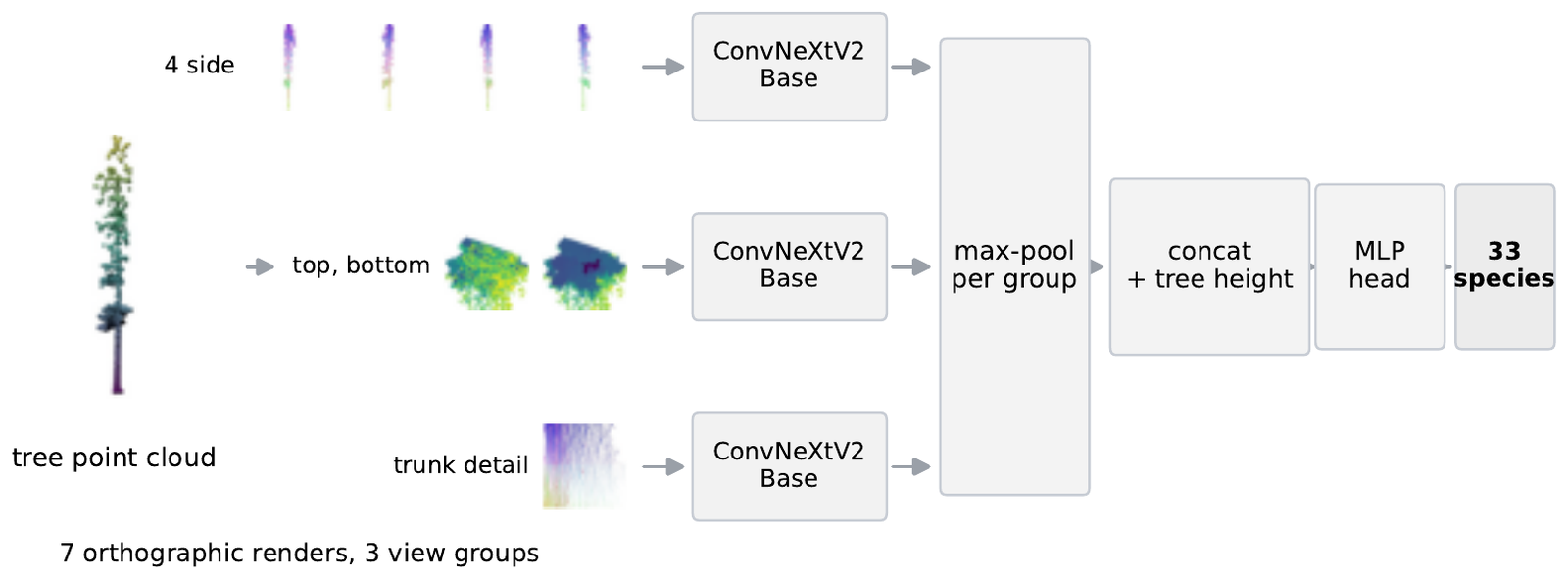
mvtree/model.py is short. The seven renders are split into three groups, each with its own ImageNet-pretrained ConvNeXtV2-Base (convnextv2_base.fcmae_ft_in22k_in1k from timm):
- the 4 side views go through one backbone, and their 1,024-d features are max-pooled across the views;
- top and bottom go through a second backbone, max-pooled the same way;
- the trunk slice goes through a third.
Max-pooling makes the side features indifferent to which side is labelled 0°. The three 1,024-d vectors are concatenated with one scalar, the tree height in metres, giving 3,073 inputs to a LayerNorm, a 512-wide hidden layer and a 33-way output. The height has to be fed in separately because the renderer scales every tree to fill the frame. The repo counts 264.7M parameters in total (reported); the released fp16 checkpoint for one fold is 529,481,710 bytes (measured), which is about two bytes a parameter.
The loss handles the long tail without resampling. Training uses logit-adjusted cross-entropy (Menon et al., 2021). With the logit for class and the class's share of the fold's training trees:
At inference the prior is dropped, so the learned logits have class frequency taken out and a rare species does not lose ties to a common one. Between the commonest and rarest species the offset is nats (reasoned).
The recipe (reported, configs/convnextv2_256.yaml): AdamW, 3 head-only epochs then 37 full ones, effective batch 32. Augmentation is only horizontal flips and cyclic shifts of the side views; colour jitter and mixup would corrupt channels that encode geometry.
Inference averages a lot. Each fold model's softmax is averaged over 20 augmented passes, then over 5 fold models, then across the 256 and 512 px models. That is 200 forward passes of the three-backbone network per tree (reasoned: 20 × 5 × 2). The repo reports about 2 s per tree on an RTX 4090.
Why pictures beat point networks here
The benchmark paper already found that the 2D multi-view methods beat the point-based ones: average OA 0.77 for image-based against 0.72 for point-based on the hidden test, with DetailView on top (reported, Puliti et al.). The hidden-test table the repo reproduces:
| Method | Input | OA % | F1 % |
|---|---|---|---|
| PointAugment + DGCNN | points | 68.3 | 70.3 |
| PointMixer | points | 71.1 | 71.1 |
| MinkNet | points | 73.7 | 72.3 |
| Ensemble PointNet++ | points | 75.6 | 74.9 |
| SimpleView | images | 76.2 | 75.6 |
| YOLOv5 | images | 77.9 | 77.3 |
| DetailView | images | 79.5 | 78.0 |
| Lee and Benes, 256 px | images | 84.0 | 83.0 |
| Lee and Benes, 256 + 512 px | images | 85.0 | 85.0 |
Hidden-test scores, reported by the authors and the benchmark. Point Transformer is not among the benchmark's baselines, so there is no number for it.
Neither paper runs a controlled experiment on why, so what follows is reasoned, not shown:
- Pretraining. ConvNeXtV2-Base arrives with ImageNet-22k features; 17,707 trees is a small training set to learn geometry from scratch.
- No subsampling. Point networks usually train on a fixed number of sampled points. The density channel counts every point, so a 150,000-point scan is not cut down first.
- Fixed scale, separate height. Filling the frame normalises size; height comes back as one clean number.
The repo's own ablation shows the backbone matters even with the input held fixed. On the public set, with the same seven renders and the same three-group design, DenseNet-201 reaches 0.818 OA and DINOv2-Base 0.819, against 0.886 for ConvNeXtV2-Base (reported, and I recomputed all three from the released predictions: 0.818, 0.819 and 0.886, measured). So the step from DetailView to this model is mostly a better backbone, the loss and a heavier ensemble on the same rendering idea. That is useful engineering, not a new representation.
Checking 85.0% and "first"
The hidden-test labels are not public, so nobody outside the organisers can recompute 85.0%. What I could check:
The leaderboard. Codabench's public API for competition 3667, "FOR-species20K benchmark", returned 22 ranked entries on 19 October (measured). The top one, submitted 30 May 2026 by the account doyouknowpete, reads OA 0.85, P 0.89, R 0.83, F1 0.85: exactly the authors' row. I cannot tie the account name to the authors, but no other entry matches those four numbers. So first holds, with two caveats:
- The leaderboard prints two decimals, so "85.0%" is "0.85". The third digit comes from the authors.
- "Previous best 79.5%" is the best published result, DetailView (the organisers' own entry reads 0.79). The leaderboard already had an entry at 0.83 OA from 2 February 2026 and one at 0.82 from 26 May, both before the authors' 30 May submission; a second 0.83 arrived in September. The margin over the field is 2 points of OA, not 5.5 (reasoned from the leaderboard values).
What was submitted. The repo ships the two submitted CSVs. Both have 2,255 rows and predict all 33 species; they agree on 95.9% of trees (measured). Both blend in a LightGBM model on 105 handcrafted geometric features, with weight 0.15 in the 85.0% file (reported). The paper describes and analyses the image model alone; the repo says the blend changes public-set accuracy by less than 0.001, which I have no way to check on the hidden test.
The downloadable 512 px weights did not score 85.0%. The originals were not kept and were retrained; 97.4% of hidden-test predictions are unchanged (reported). The README says so plainly.
Public-set numbers. From results/oof/convnextv2_256_random.npz, the out-of-fold predictions for all 17,707 public trees, I get OA 0.886 and macro-F1 0.843, matching the paper's Table 2 as the repo quotes it, and 0.879 / 0.934 / 0.894 OA on TLS / MLS / ULS trees (measured, all matching). Mean per-species accuracy (balanced accuracy) is 0.846 (measured), which is the number to put next to the hidden test's 84.0% for the same 256 px model. By LiDAR type on the hidden test the authors report 85.6% (TLS), 93.4% (MLS) and 79.2% (ULS).
Per-species: where the model is right
The per-species chart, computed from the same out-of-fold file, is where the benchmark starts to tell on itself (all measured):
- The weakest classes are Fraxinus excelsior at 39.7%, Euonymus europaeus 54.8%, Ulmus laevis 55.4% and Tilia cordata 64.4%. Six of the ten weakest come from one dataset, BlueCat_a, a dense TLS plot of mixed broadleaves with nine species. The authors make the same observation: co-occurring deciduous species in dense mixed forest (Acer, Carpinus, Fraxinus, Ulmus, Tilia, Euonymus) account for about half of the remaining errors (reported).
- The eight best classes, all at 96.4% or above, each occur in one source dataset only: Corylus avellana, Picea glauca, Pinus radiata, Populus tremuloides, Eucalyptus miniata, Pinus contorta, Pinus resinosa and Acer saccharum.
- Group the species by how many species share their main source. The 11 species whose main source holds three species or fewer average 96.3% accuracy; the other 22 average 78.7%.
That last split is a correlation and not proof; small sources also tend to be conifers scanned cleanly. But it is what you would expect if part of what the model recognises is the scan rather than the tree. If a Pinus radiata only ever arrives from one drone survey, any drone-survey signature is a perfectly good Pinus radiata detector on a random split.
The paper's real result: same species, unseen source
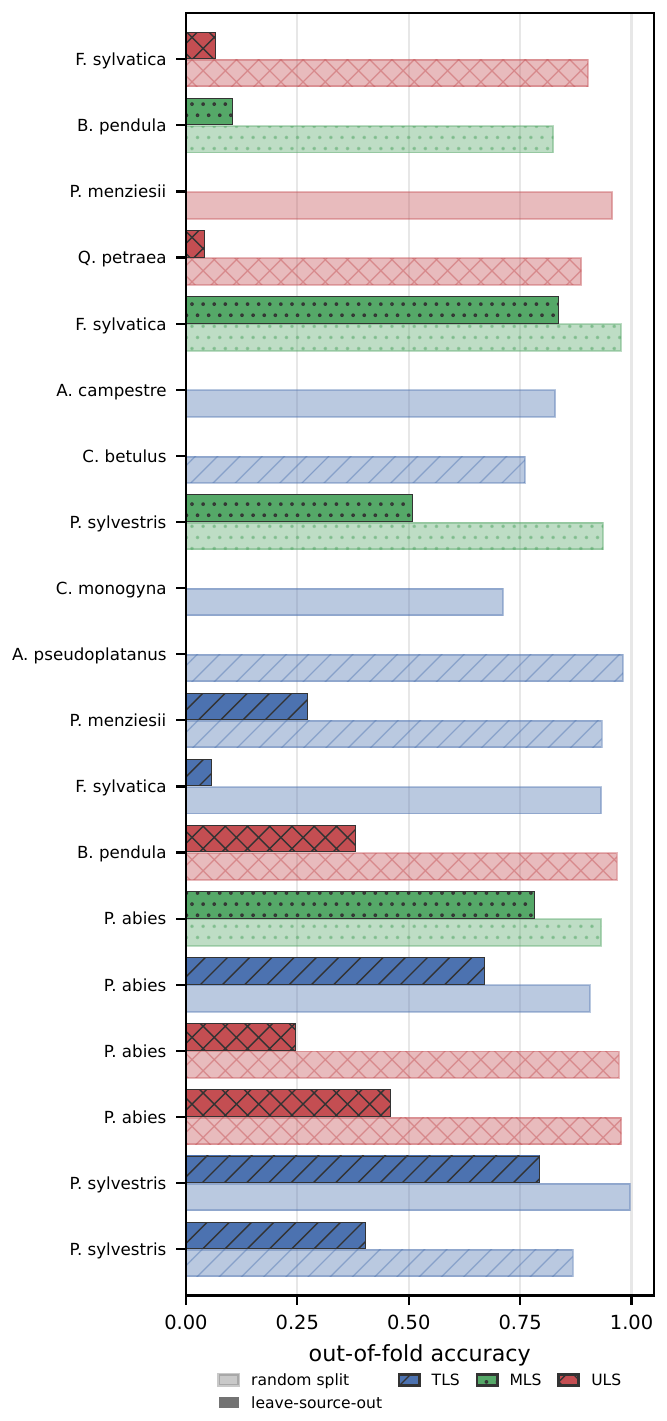
The authors test that with a source-species holdout. Split the 25 sources into five groups. For fold k, remove from training the trees in group k of every species that also occurs outside it, and score exactly those trees. The species stays in training from other sources; only the (source, species) pair is new. A cell counts only if the species keeps at least 50 training trees of the same LiDAR type and has at least 20 held-out trees, so "new source" is not confused with "less data".
Each scored tree is predicted by the random-split model and by the holdout model: same trees, only the split differs. I reimplemented the scoring on the released convnextv2_256_source_holdout.npz and got their numbers exactly (measured):
| Trees | Random split | Unseen source | |
|---|---|---|---|
| Tree-weighted | 5,566 | 94.8% | 60.2% |
| Mean over 8 species | 8 species | 81.5% | 36.0% |
Pinus sylvestris holds at 69.1% and Pseudotsuga menziesii at 69.8%; Betula pendula falls from 91.0% to 24.8%; Acer pseudoplatanus from 79.2% to 0.0% (measured, on 24 trees). Without the support filter, over all 13,497 held-out trees, accuracy goes from 89.7% to 30.1% (measured), but that includes cells where a species almost disappears from training, which is exactly what the filter is there to exclude.
The controls, all reported:
- Not a data-size effect. Removing the same number of trees per species and LiDAR type at random across sources keeps 94.1% accuracy on the same cells, against 44.8% for the source-structured removal in that fold.
- Not one leaky dataset. Dropping the held-out source datasets entirely changes the drop only from 42 to 37 points.
- The source is in the outputs. A logistic regression predicts which of the 25 datasets a tree came from, using only the model's 33 species probabilities, with 69% accuracy (chance 4%).
- Not specific to this benchmark. On PureForest, a separate airborne-LiDAR species dataset, holding out whole forests costs 9 points under matched support.
- Not specific to this backbone. DINOv2-Base drops 43.0 points and DenseNet-201 39.7, against ConvNeXtV2's 34.5.
So the first-place model is also the best of the three across sources, and it still loses over a third of its accuracy on a source it has not seen for that species. The random split rewards learning the scanner and the site, and that applies to every entry on the leaderboard.
Running it
The code ships a CLI (./predict.sh tree.laz), a self-hosted web app (mvtree serve) that keeps records you can check against field identifications, and an offline Android app. On a shared 4-core cloud VM (Xeon at 2.80 GHz, CPU only, 2 threads) I installed CPU PyTorch in a Python 3.12 venv, downloaded fold 0 of the 256 px model (529,481,710 bytes, SHA-256 matching the manifest) and ran the repo's Predictor on the four example scans. Fold 0 did not train on two of them (00415, 05554); it did train on the other two.
| Scan | Held out by fold 0 | Top-1, 1 pass | Time, 1 pass | Time, 20 passes |
|---|---|---|---|---|
| Picea abies, TLS, 115,626 pts | yes | Picea abies, 1.00 | 4.2 s | 76.3 s |
| Pinus sylvestris, ULS, 53,839 pts | yes | Pinus sylvestris, 1.00 | 5.9 s | 79.3 s |
| Fagus sylvatica, TLS, 142,187 pts | no | Fagus sylvatica, 1.00 | 3.1 s | 63.2 s |
| Quercus robur, MLS, 150,574 pts | no | Quercus robur, 1.00 | 3.3 s | 98.5 s |
Measured. Model load 6 to 10 s; peak resident memory 4.2 GB.
All four are right, with the second choice below one in a million. Two held-out trees is not an accuracy estimate; the 88.6% out-of-fold figure above is. The full paper ensemble runs ten fold models at 20 passes each, so on this VM it would take roughly ten times the 20-pass column, around 10 to 16 minutes a tree (reasoned). On CPU, use --folds 0 --tta 1: one model, one pass, a few seconds.
The phone app runs that configuration with every MatMul quantised to 8-bit, 1,016 MB down to 294 MB. The repo reports 0.8907 OA on fold 0's 3,542 held-out trees against 0.8905 for fp32, and about 4 s a tree on an 8-core emulator; it has not been timed on a phone. I found Kotlin source and build steps but no prebuilt APK, so expect to export the model and build it yourself.
Licences
- Code: GPL-3.0-or-later (the repo's
LICENSE). - Data: FOR-species20K is GPL-3.0-or-later on its Zenodo record (measured from the record's metadata). That includes the four example scans in the repo.
- Weights: on Google Drive, 5.3 GB for both resolutions. The README states they were trained on the GPL data and does not give them a separate licence; treat them as GPL-3.0-or-later too unless the authors say otherwise.
- Android app: GPL code plus ONNX Runtime (MIT) and laszip4j (LGPL-2.1).
What I would use it for
As a field tool for the benchmark's species and forests, it is ready: the CLI and the web app's records page are what an inventory team needs to check a model against its own plots. As evidence that LiDAR species recognition is solved at 85%, it is not, and the authors say so: validate on local reference trees before trusting a new sensor, region or protocol. It is also a closed set of 33 mostly European species with no "unknown" class.
If you work on point clouds, the useful part is the protocol: splits/source_holdout_5fold.csv and the scoring script take any model's out-of-fold probabilities, and I would like to see the point networks run through it. Related here: Invaria, a point-cloud encoder built not to care how the cloud was sampled; FAST-LIO2, how mobile scans get registered; Hesai Kosmo, a handheld lidar that makes this kind of data; SpatialLM, 3D structure read by a model built for something else; and the Hilti SLAM datasets, a benchmark graded against surveyed ground truth.