BM25: the ranking function that refuses to die

Here's a fact that should be more embarrassing for machine learning than it is: a ranking function designed in the early 1990s, with no learned parameters and no notion of meaning, is still the default text scorer in Lucene, Elasticsearch, and OpenSearch — and still a baseline that dense neural retrievers regularly fail to beat out of domain. It's called BM25, and if you do search, retrieval, or RAG, it's worth understanding exactly, because you're almost certainly running it.

"BM25" is Best Matching 25 — roughly the 25th matching function tried in the Okapi information-retrieval project at City University London (Robertson, Spärck Jones, and colleagues), grounded in the probabilistic relevance framework. Strip away the theory and it's a small, honest idea: score a document by summing, over the query terms it contains, how rare each term is times how emphatically the document uses it — with two corrections that make it work in practice. Let's build it.

Start with TF-IDF, and its two flaws

The classic bag-of-words score is TF-IDF: for each query term, multiply its frequency in the document (term frequency, TF — "this document uses the word a lot") by its rarity across the corpus (inverse document frequency, IDF — "and the word is distinctive"). Sum over query terms. It's a reasonable instinct, and it has two clear problems:

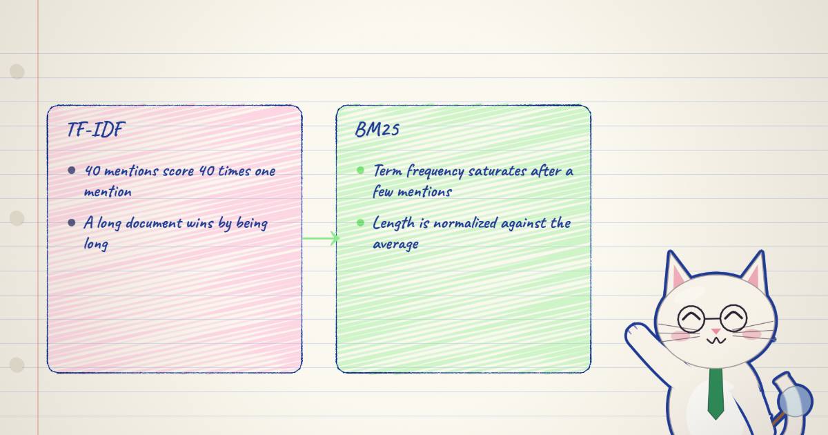
1. TF grows linearly and forever. A document that says "jaguar" 40 times scores 40× one that says it once. But the difference between 1 and 2 mentions is meaningful; the difference between 39 and 40 is noise. Relevance saturates.
2. Length is unaccounted for. A 10,000-word document will rack up term counts just by being long, drowning out a tight 100-word document that's genuinely more on-topic.

BM25 is, almost exactly, TF-IDF with those two flaws fixed. Here's the whole thing:

Three pieces do all the work: the IDF weight, the saturating term-frequency factor (the $k_1$ part), and the length normalization (the $b$ part). Here they are, color-coded — the map for the rest of the piece:

Take them one at a time.

Rarity: the IDF term

$f(q,D)$ is just the count of term $q$ in document $D$. The multiplier in front is inverse document frequency — how much a term's presence should count, based on how rare it is:

$N$ is the number of documents, $n(q)$ the number containing $q$. A term in every document (like "the") gets an IDF near zero — matching it tells you nothing. A term in one document out of a million gets a large IDF — matching it is almost the whole story. This is why BM25 needs no stopword list: common words are down-weighted automatically because their IDF collapses. (The $\ln(1 + \cdots)$ form is Lucene's; it keeps IDF non-negative. The original Robertson–Spärck-Jones IDF drops the $+1$ and can go slightly negative for terms in more than half the corpus.)

Saturation: the k1 term

Now the first fix. Instead of using the raw count $f(q,D)$, BM25 passes it through a saturating function $\frac{f\,(k_1+1)}{f + k_1\cdot(\dots)}$ that rises fast for the first few occurrences and then flattens toward an asymptote. The parameter $k_1$ controls how fast:

The first mention of a term is strong evidence; each additional mention adds less. That curve — not the straight line of TF-IDF — is how relevance actually behaves. Set $k_1 = 0$ and it becomes binary (any occurrence counts the same); crank $k_1$ up and it straightens back toward linear TF. Lucene's default is $k_1 = 1.2$.

Length: the b term

The second fix lives in the denominator: the $k_1$ term is scaled by $\left(1 - b + b\,\frac{|D|}{\text{avgdl}}\right)$, where $|D|$ is the document's length and $\text{avgdl}$ the average across the corpus. A longer-than-average document gets a bigger denominator, so its term-frequency factor is discounted — the same two mentions count for less when they're diluted across more text:

The knob $b \in [0,1]$ sets how aggressively. At $b = 0$ length is ignored entirely; at $b = 1$ it's fully normalized. The default $b = 0.75$ is a compromise that's proven hard to beat.

Put it together: a live BM25 engine

That's the entire algorithm. Here it is running on a tiny corpus — edit the query, drag $k_1$ and $b$, and every document is re-scored with the exact formula above. Expand a document to see each query term's contribution (its IDF times the saturated, length-normalized factor):

Notice the behaviors fall out on their own: rare query terms dominate the ranking, repeating a common word barely moves the score, and a long document doesn't win just for being long. No training, no embeddings — just term statistics arranged sensibly.

Thirty lines of Python

There's no magic hiding in a library. The whole thing is a couple of counters and the formula:

import math
from collections import Counter
 
class BM25:
    def __init__(self, corpus, k1=1.2, b=0.75):
        self.k1, self.b = k1, b
        self.docs = [doc.lower().split() for doc in corpus]
        self.N = len(self.docs)
        self.avgdl = sum(len(d) for d in self.docs) / self.N
        self.tf = [Counter(d) for d in self.docs]          # term counts per doc
        self.df = Counter()                                 # docs containing each term
        for d in self.docs:
            for term in set(d):
                self.df[term] += 1
 
    def idf(self, term):
        n = self.df.get(term, 0)
        return math.log(1 + (self.N - n + 0.5) / (n + 0.5))
 
    def score(self, query, i):
        d, tf = self.docs[i], self.tf[i]
        norm = self.k1 * (1 - self.b + self.b * len(d) / self.avgdl)
        s = 0.0
        for term in query.lower().split():
            f = tf.get(term, 0)
            if f:
                s += self.idf(term) * f * (self.k1 + 1) / (f + norm)
        return s
 
    def rank(self, query):
        return sorted(((i, self.score(query, i)) for i in range(self.N)),
                      key=lambda x: -x[1])

In production you don't loop over every document — you keep an inverted index (term → postings list of documents that contain it) and only score documents that share a term with the query. That's what makes BM25 fast enough to serve web-scale corpora on commodity hardware, and it's the same index that's been powering Lucene since 2011.

The variants you'll meet

The core formula spawned a small family, mostly patching edge cases:

• BM25+ adds a small constant $\delta$ (default 1.0) to the term-frequency factor, fixing a subtle bug where very long documents can be over-penalized to the point that a document containing a rare term scores below one that doesn't.
• BM25F ("fielded") scores structured documents — title, body, anchor text — by combining per-field term frequencies before saturation, with a weight per field, so a title match counts more than a body match. It's what real search engines actually run.
• BM25L re-weights to stop long documents from being unfairly buried.
• Lucene's implementation is BM25 with the non-negative IDF above and per-field length norms quantized into a single byte — the pragmatic engineering version of the equation.

Why it won't die

Neural retrieval was supposed to make this obsolete years ago. It hasn't, for reasons worth naming:

• It's a brutal baseline. On out-of-domain benchmarks (the BEIR suite made this famous), BM25 beats or ties many dense retrievers — because it can match any term, including names, codes, and jargon a fixed-vocabulary embedding never saw in training. It never has an "out-of-distribution" moment.
• It's the sparse half of hybrid search. The current default in serious systems is to run BM25 and a dense retriever and fuse the results (often with reciprocal-rank fusion). Lexical precision plus semantic recall beats either alone, which is why "BM25 is obsolete" quietly became "BM25 is one of your two retrievers."
• It's cheap and interpretable. No GPU, no training, no embedding drift. When it ranks a document highly you can point at exactly which rare terms did it — which matters when a ranking has to be debugged or defended.

The lesson I take from BM25 is that a model doesn't have to learn anything to encode real knowledge about a problem. Every piece of it is a hypothesis about relevance — rarity matters, repetition saturates, length dilutes — written as arithmetic instead of learned from data. Three good hypotheses, two tunable knobs, and thirty-five years later it's still the thing your search bar is probably running.

BM25 originates in the Okapi project (Stephen Robertson, Karen Spärck Jones, et al.) and the probabilistic relevance framework; the formulation and non-negative IDF here follow Lucene's BM25Similarity (defaults $k_1 = 1.2$, $b = 0.75$). BM25+ / BM25L are from Lv & Zhai (2011).