UNREAL: one frozen LLM as both the retriever and the long-context filter

2026-10-08 · 29 min · retrieval · long-context · sparse-attention · benchmarks · inference

Why read this

Traces each UNREAL headline to its baseline, recomputes parameters, index bytes and FLOP break-even from configs, and maps it against sparse attention.

Original analysis
A lasting reference
A new technique

Inference & servingNeeds datacenter GPUsPractitioner paper

How this was scored

Is it new?: 2 of 3: A real new idea, method or capability
Can I trust it?: 2 of 3: Measures key facts from files, code or configs
Can I run it?: 0 of 3: Closed, nothing to run
Will I understand it?: 2 of 3: Mechanism from first principles with figures
Can I act on it?: 2 of 3: A concrete recipe, numbers or comparison
Will it last?: 2 of 3: A reference for a year or more
Does it affect many?: 1 of 3: A specialist community
Only here?: 2 of 3: A teardown or measurement few others did

Score 59 of 100, ranked 265 of 476 rated articles. Each question is answered 0–3 by hand, and a 3 is rare. How articles are scored

A RAG system and a long-context model are both answering the same question: which few pieces of all this text matter for the question in front of me? A retriever answers it out loud, with a separate embedding model, an index and a top-k. A long-context model answers it silently, inside attention, and tends to get worse at it as the haystack grows. Production stacks end up running both, and keeping two models aligned.

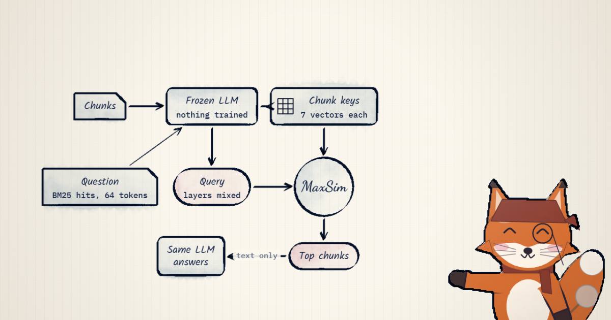
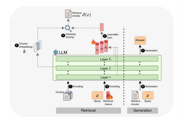
UNREAL, from Edan Kinderman, Elad Hoffer, Yochai Blau, Brian Chmiel, Ron Banner, Daniel Soudry and Boris Ginsburg (all NVIDIA; Soudry is also at the Technion), says you can make the generator itself do the explicit version. Freeze the LLM. Read its hidden states to get chunk keys. Append 64 learned tokens to the question, read the hidden states at those positions to get a query, score every chunk, keep the top few, and hand their text back to the same LLM. Fewer than 500K trainable parameters. The abstract reports HotpotQA recall going from 49.1% to 73.2% on a 21M-chunk Wikipedia index, and NoLiMa accuracy going from 1.0% to 24.83% at 128K tokens.

That second number is what sent me in. A 1.0% baseline at 128K is the kind of number that says more about the baseline than the method. So I read the paper end to end, appendices included, pulled the configs of every backbone it names from Hugging Face, and redid the arithmetic it leaves implicit. There is no code release and no weights for the trained module; I looked for both and found neither, so everything below comes from the paper, the configs and my own arithmetic.

The short version: the mechanism is simple and well-motivated, and the corpus retrieval results are strong even after you account for what the baselines did not get. The long-context headline compares against the weakest line on its own chart. And "unified" means one set of weights and one scoring rule used in two quite different pipelines, which is still a useful thing to have.

Three line charts, one per backbone (Nemotron-3.5-Lightning-30B-A3B, Qwen3.5-35B-A3B, Muse-Glimmer-30B), plotting exact match against context length from 8K to 100M tokens on a log axis. A dashed line separates a long-context region up to about 1M from a RAG region beyond. Full-context reading falls steeply and stops at 256K to 512K. BM25 declines steadily. Embedding-plus-reranker baselines track UNREAL up to about 128K and fall below it after. UNREAL stays highest from roughly 32K to 100M. — The paper's opening chart: the same question answered from 8K to 100M tokens of padded Wikipedia. Full-context reading stops where it became infeasible to run; the retrieval methods keep going. Note how close the external retrievers stay to UNREAL below 128K (paper, Figure 1).

Two scales of one operation

The paper's framing is the part I would keep even if the numbers were weaker. At long-context scale, evidence selection is implicit: the model receives everything and has to suppress what is irrelevant while it generates. At corpus scale it is explicit and external: a retriever picks passages before generation starts. The operation is the same, query-conditioned selection over chunks; only the count changes, from hundreds of chunks in a prompt to millions in a corpus.

If that is right, the two should be served by one mechanism, and the natural place to put it is inside the model that will read the evidence, so chunks are ranked in the representation space of their eventual reader. And the selection should be explicit, so distractors are actually removed before generation rather than merely down-weighted.

UNREAL is the decoder-only successor to INTRA (arXiv 2605.05806), the same group's earlier paper, which retrieved from the encoder memories of an encoder-decoder model through its cross-attention. Decoder-only models have no separate encoder and no cross-attention, so both halves had to be rebuilt from things a decoder does have: its residual stream.

How a hidden state becomes a key

Start with the chunk side, because it is the simpler one. Take a chunk $c_i$ of $T_i$ tokens, run it through the frozen LLM on its own, and stop at one intermediate layer $\ell_c$ . The residual-stream states at that layer are the chunk's representation:

k_i = \mathrm{LLM}_{\ell_c}(c_i) \in \mathbb{R}^{T_i \times d}

where $d$ is the model's hidden size. One vector per token is too much to store for 21M chunks, so the token states are split into $L_p$ contiguous groups and each group is mean-pooled. The paper uses $L_p = 7$ : every chunk becomes seven $d$ -wide vectors, whatever its length (the Wikipedia chunks are about 141 tokens).

Which layer? The paper picks it on a dev set, motivated by prior work showing intermediate layers carry richer semantics than the last one. The chosen layers are $\ell_c = 27$ of 40 for Qwen3.5-35B-A3B, 47 of 52 for Muse-Glimmer-30B and 42 of 52 for Nemotron-3.5-Lightning-30B-A3B. I checked these against each model's config.json. In zero-based layer indices, 27 is one of Qwen3.5-35B-A3B's ten full-attention layers (3, 7, 11, …, 39; the other thirty are linear attention), 47 is one of Muse-Glimmer's thirteen global-attention layers (the other 39 use a 2,048-token sliding window), and 42 is the last of Nemotron-3.5-Lightning's six attention layers (5, 12, 19, 26, 33, 42; the rest are Mamba and MoE blocks). So in all three the index is read just after a global-attention block, late in the stack.

What surprised me is that it barely matters. The layer ablation for Nemotron-3.5-Lightning (Table 4) tries layers 8, 18, 30, 38, 42 and 48, and complete-evidence recall@10 on HotpotQA stays between 69.42 and 72.93 across all of them. Layer 8 gives 70.25. Whatever makes this work is not a magic layer.

The query side, and where the 500K parameters live

The query is where the learning happens. UNREAL builds a retrieval input

x_{\mathrm{ret}} = \bigl[\,C_0(x),\; x_1, \dots, x_{T_q},\; \rho_1, \dots, \rho_R\,\bigr]

with three parts. $C_0(x)$ is the top five BM25 chunks for the question. Then the question's own tokens. Then $R = 64$ learned embeddings $\rho_1 \dots \rho_{64}$ , which are not words; they are free $d$ -dimensional vectors fed in where token embeddings would go. A single further learned vector sits at the very start of the sequence as a soft prompt; it is never read out, it only nudges the frozen model into "retrieval mode".

Because the retrieval tokens come last, the causal mask lets each of them attend to the BM25 context and the question. Their residual states, read at every full-attention layer $\ell$ , are the raw query:

q_\ell(x_{\mathrm{ret}}) = \bigl[\mathrm{LLM}_\ell(x_{\mathrm{ret}})\bigr]_{\text{last } R \text{ positions}} \in \mathbb{R}^{R \times d}

The layers are mixed with learned scalars $\alpha_\ell$ , the 64 rows are mean-pooled into $G = 4$ groups, and each chunk is scored with ColBERT's late-interaction MaxSim:

s_i = \mathrm{MaxSim}\Bigl(\textstyle\sum_\ell \alpha_\ell\, q_\ell,\; k_i\Bigr), \qquad \mathrm{MaxSim}(u, v) = \sum_a \max_b \langle u_a, v_b \rangle

For each of the four query vectors, find the best of the chunk's seven vectors, and add the four maxima. The top $n$ chunks by $s_i$ are the selection.

Notice the asymmetry. The key comes from one layer; the query is a weighted mix of all the full-attention layers, six of them for Nemotron, ten for Qwen3.5-35B-A3B, thirteen for Muse-Glimmer. That works because a residual stream is a shared workspace that every layer adds into, so states from different depths live in roughly comparable coordinates. It also explains why the method reaches across architectures: it never touches an attention head's queries or keys, so a Mamba or Gated DeltaNet block is as readable as a softmax one. That is a quiet but real advantage over every method that scores chunks with attention internals.

Method diagram. Left: chunks are encoded by the frozen LLM (a stack labelled Layer 1, Layer l, Layer L) and chunk embeddings k are read from layer l. Middle: the query x and trainable retrieval tokens rho are encoded; their states q1, ql, qL at several layers are combined by a learnable sum with weights alpha, both marked trainable with a flame icon. A similarity-scoring step compares the summed query to the chunk embeddings and retrieves chunks S(x). Right, after a dashed divider: generation, where the retrieved chunks and the query are fed to the same LLM to produce an answer. Steps are numbered 1 to 7. — UNREAL in one picture. Only the retrieval tokens ρ and the layer weights α train (the flames); the LLM is frozen. Retrieval and generation are two separate passes through the same model (paper, Figure 2).

The paper gives the parameter count as $(R+1)D + |\alpha|$ : 64 retrieval vectors plus one soft prompt, each $D$ wide, plus one weight per mixed layer. With the hidden sizes from the configs and one $\alpha$ per full-attention layer, that is

Qwen3.5-35B-A3B: $65 \times 2048 + 10 = 133{,}130$
Qwen3.5-4B: $65 \times 2560 + 8 = 166{,}408$
Nemotron-3.5-Lightning-30B-A3B: $65 \times 2688 + 6 = 174{,}726$
Muse-Glimmer-30B: $65 \times 6656 + 13 = 432{,}653$

So the Nemotron module is 174,726 trainable numbers. All four are under 500K, and the largest is about $1.4 \times 10^{-5}$ of a 30B model, inside the paper's "less than $2\times 10^{-5}$ ". The paper states the Nemotron count of six mixed layers directly; for the others I assumed one weight per full-attention layer, which is what "a learnable sum of the full-attention outputs" implies.

Training: contrastive, with hard negatives from BM25

The loss is multi-positive InfoNCE. For a question $x$ with oracle chunks $\mathcal{O}(x)$ (the chunks that contain the annotated evidence) and a pool $\mathcal{B}(x)$ of oracles plus hard negatives:

\mathcal{L} = -\frac{1}{|\mathcal{O}(x)|} \sum_{j \in \mathcal{O}(x)} \log \frac{\exp(s_j / \tau)}{\sum_{i \in \mathcal{B}(x)} \exp(s_i / \tau)}

Every oracle should outscore everything in the pool. The interesting part is where the negatives come from. For each question, the oracle chunks themselves are used as BM25 queries against the corpus; the top ten hits are thrown away because they are usually near-duplicates of the oracle, and the next 500 become hard negatives. Within a microbatch the negatives of all questions are pooled and deduplicated, with care that one question's oracle is never another's negative for that same question. These are chunks that look lexically like the evidence and are not, which is exactly the confusion a frozen model's default similarity makes.

The data is the training splits of eight Wikipedia QA sets (Natural Questions, SQuAD v2, HotpotQA, 2WikiMultiHopQA, MuSiQue, IIRC, FEVER, HoVer), all remapped onto the 21M-chunk DPR Wikipedia-2018 corpus by a KILT-style title-and-overlap alignment. Then 15K steps at a global batch of 256 questions, AdamW with $\beta = (0.9, 0.95)$ , weight decay 0.1, 100 warmup steps, learning rate $5\times10^{-3}$ or $10^{-2}$ . Only $\rho$ , the soft prompt and $\alpha$ get gradients. The LLM never changes, which is the whole point: the model that generates is bit-for-bit the model you downloaded.

What the ablations say is doing the work

Table 3 of the paper changes one design choice at a time on Nemotron-3.5-Lightning. The column I care about is complete-evidence recall@10 on HotpotQA, baseline 72.93:

change	HotpotQA all-R@10	drop
no BM25 context ( $\lvert C_0 \rvert$ 5 → 0)	56.73	16.20
read one layer instead of mixing all six	61.01	11.92
16 retrieval tokens instead of 64	67.83	5.10
one query group instead of four	68.37	4.56
one BM25 chunk instead of five	68.83	4.10
one pooled vector per chunk instead of seven	69.11	3.82
100 hard negatives instead of 500	70.59	2.34
no soft prompt	70.86	2.07

The largest single contributor is BM25. Without the five BM25 chunks in front of the question, the method loses 16.2 points. I read this as pseudo-relevance feedback doing the job of a first hop. A two-hop question like "which instrument does the lighthouse keeper's sister play" does not name the keeper. BM25 on "lighthouse" finds the chunk that does, the retrieval tokens attend to it, and now the query can go looking for the sister by name. The interactive below reproduces this on a toy example. The second-largest contributor is the multi-layer read-out, which is the actual new idea. The fiddly knobs (token count, groups, negatives, soft prompt) are each worth two to five points.

There is one more experiment that changes how I read the paper's title. Appendix A.2.1 asks whether a frozen model retrieves at all without training: mean-pool each chunk's attention keys and the question's attention queries per head, dot them, average over heads, rank. That is the "retrieval heads" style of evidence. On NoLiMa with Nemotron-3-Nano it does beat random, but not by much: the best layer reaches an average recall@10 of about 0.24 against roughly 0.04 for random, while trained UNREAL gets about 0.65.

Two charts. Left: NoLiMa accuracy and average recall against the number of retrieved chunks n on a log axis from 1 to 50 plus M (all chunks). Recall rises steadily from about 0.3 to about 0.86 and to 1.0 at M. Accuracy rises from about 29% at n=1 to a peak near 58% around n=12, then falls to about 39% at n=50 and about 20% at M. Right: average recall@n against n for untrained per-layer attention scoring (thin lines), the best untrained layer L5 (bold blue), UNREAL trained (green) and random (dashed). At n=10 UNREAL is about 0.65, best untrained layer about 0.24, random about 0.04. — Left: the inverted U. More chunks raise recall and, past about a dozen, start to hurt accuracy. Right: untrained attention scores from the frozen model retrieve better than random, and trained UNREAL is far ahead of both (paper, Figure 6).

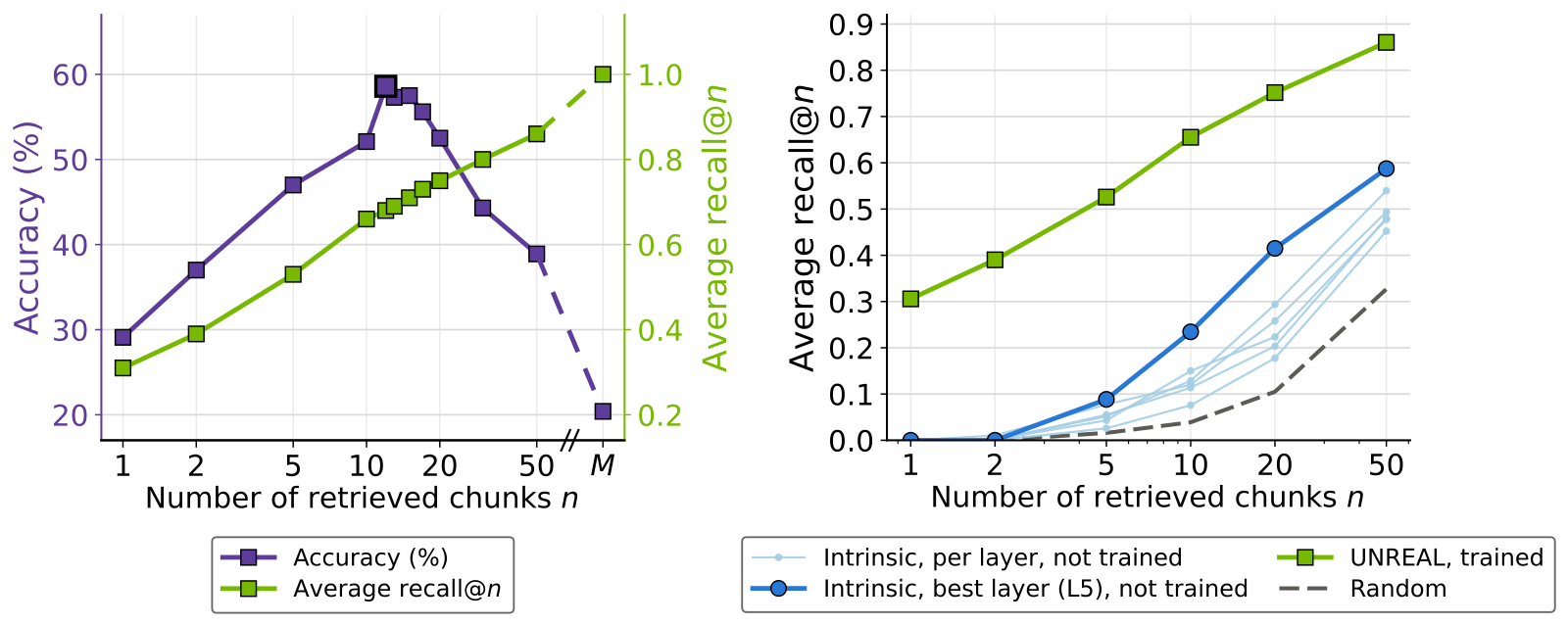
So the "intrinsic capability" is a weak signal that 64 trained vectors amplify a lot. That is a fine result. It is also a reminder that the retrieval here is learned, on in-domain supervision, not discovered.

Checking the corpus numbers

On the full 21M-chunk index, the paper reports complete-evidence recall@10: a question only counts if every annotated evidence chunk is in the top ten. For multi-hop questions that is a harsh metric, which is part of why the absolute numbers look low.

Nine bar-chart panels of complete-evidence recall@10 on 21M Wiki-2018 chunks: HotpotQA, 2WikiMultiHopQA, MuSiQue, HoVer, IIRC, SQuAD v2, FEVER, Natural Questions and the average over 8 datasets. Eleven bars each: BM25, BGE-large-en-v1.5, Qwen3-Emb-0.6B, Qwen3-Emb-4B, Hybrid RAG, LateOn plus reranker, Qwen3-Emb-4B plus reranker, and four UNREAL backbones. HotpotQA: best baseline 49.1, UNREAL 69.1, 70.5, 73.2, 72.9. 2Wiki: best baseline 31.7, UNREAL up to 60.1. MuSiQue: 8.8 to 14.4. Natural Questions: best baseline 26.7, UNREAL 24.9 to 30.6. Average: best baseline 36.5, UNREAL 45.7 to 49.6. — Complete-evidence recall@10 across eight datasets. The multi-hop sets (red titles) carry the big gains; on single-hop Natural Questions the 4B UNREAL is below an off-the-shelf 4B embedder (paper, Figure 3).

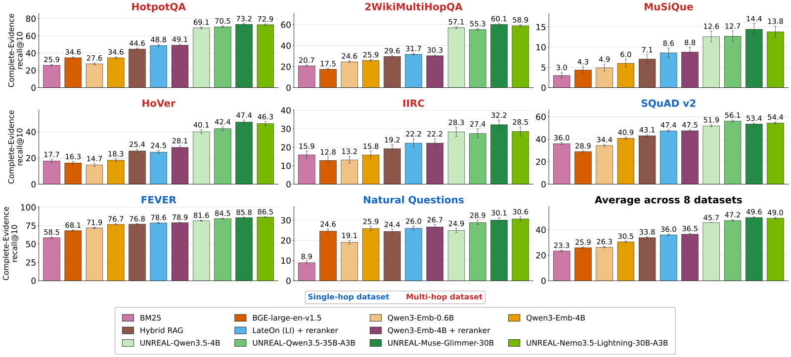
Reading the bars off the paper's chart:

HotpotQA, 49.1 → 73.2. The 49.1 is Qwen3-Embedding-4B followed by the Jina reranker, the strongest baseline. The 73.2 is UNREAL on Muse-Glimmer-30B, a 30B dense model.
2WikiMultiHopQA, 31.7 → 60.1. Here the 31.7 is a different baseline, LateOn (a ColBERT-style multi-vector retriever) plus reranker; Qwen3-Embedding-4B plus reranker is 30.3. The 60.1 is again Muse-Glimmer.
MuSiQue, 8.8 → 14.4, same pattern.
Averaged over all eight datasets, 36.5 for the best baseline against 49.6 for the best UNREAL.

Each headline picks the best baseline for that dataset and the best UNREAL backbone, which is the normal way to report it. The comparison that actually convinced me is a different one: UNREAL on Qwen3.5-4B, a 4B model, gets 69.1 on HotpotQA and 57.1 on 2WikiMultiHopQA. That is the same parameter class as the Qwen3-Embedding-4B baseline, and it still gains 20 points on HotpotQA. Model size is not the explanation.

Two things keep me from taking the margins at face value. First, UNREAL is trained on the training splits of all eight evaluation datasets, mapped onto this exact corpus, with hard negatives mined from this exact corpus. The baselines are off-the-shelf. The paper points out that Qwen3-Embedding was itself trained on HotpotQA and Natural Questions, which is true, but it was not trained on 2WikiMultiHopQA's or HoVer's distribution against Wiki-2018 hard negatives. The missing control is a baseline embedder fine-tuned on the same data and negatives; without it, some of the gap is in-domain training rather than method. Second, UNREAL's query sees five BM25 chunks and the dense baselines' queries do not. Hybrid RAG fuses BM25 and dense rankings, but it does not let the BM25 hits shape the query. The ablation says that input alone is worth 16 points on HotpotQA. Remove it and Nemotron-3.5-Lightning still gets 56.73 against the baseline's 49.1, so the method survives, with a smaller margin.

Single-hop is where the gains thin out. On Natural Questions, Qwen3-Embedding-4B plus reranker reaches 26.7 and UNREAL ranges from 24.9 (the 4B) to 30.6. That fits the story: the multi-layer, BM25-conditioned query earns its keep when the question needs a bridge.

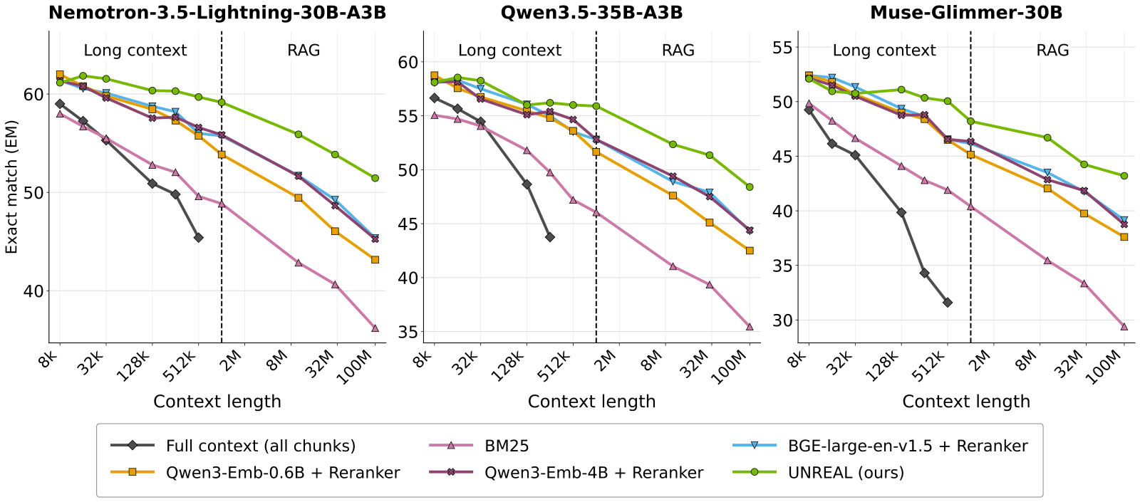
Retrieval quality carries through to answers. With Nemotron-3.5-Lightning as the generator and only the top-5 retriever varied (Table 1), HotpotQA exact match goes from 43.3 for the best baseline to 52.6 with UNREAL, against 64.3 when the model is handed only the oracle chunks. 2WikiMultiHopQA goes from 32.5 to 42.0 and MuSiQue from 13.2 to 16.9. Qwen3.5-35B-A3B as the generator shows the same ordering (48.2 against 41.3 on HotpotQA).

Inside a 128K prompt

Now the second scale. Given a long prompt, UNREAL treats it as a small corpus. It splits the text into sentence-aligned chunks of about 141 tokens that never cross a document boundary, runs each chunk through the frozen model alone up to $\ell_c$ , scores them with the same 64 retrieval tokens and the same $\alpha$ , keeps the top $n$ , reassembles those in their original document order, and generates from that much shorter prompt. No long-context training data is involved; the modules are the ones trained for corpus retrieval.

Two things about this are easy to miss. The chunks are encoded independently, so no chunk ever attends to another during selection; and the generation pass re-encodes the selected text from scratch. Nothing from the selection pass is reused as KV cache. This is RAG over your own prompt, done with your own model, not a form of sparse attention.

Two line charts. Left, NoLiMa answer accuracy from 4K to 128K tokens with Nemotron-3-Nano: oracle gold chunks near 96 throughout; UNREAL from about 93 at 4K down to about 25 at 128K; BGE-large plus reranker and Qwen3-Emb-4B plus reranker just below UNREAL, ending near 16 and 14; full context from about 63 at 4K down to about 1 at 128K; BM25 from about 31 to near 0. Right, LV-Eval F1 from 16K to 256K words with Nemotron-3.5-Lightning: full context falls from about 53.8 to about 50.0; UNREAL highest at most lengths, ending at about 54.7; BGE-large plus reranker ends at about 54.6. — NoLiMa (left) and LV-Eval (right). The headline pairs are UNREAL against full context: 1.0% to 24.83% at 128K, 49.97 to 54.66 F1 at 256K. The retrieval baselines are much closer, and at 256K on LV-Eval essentially tied (paper, Figure 4).

Whose 1.0%?

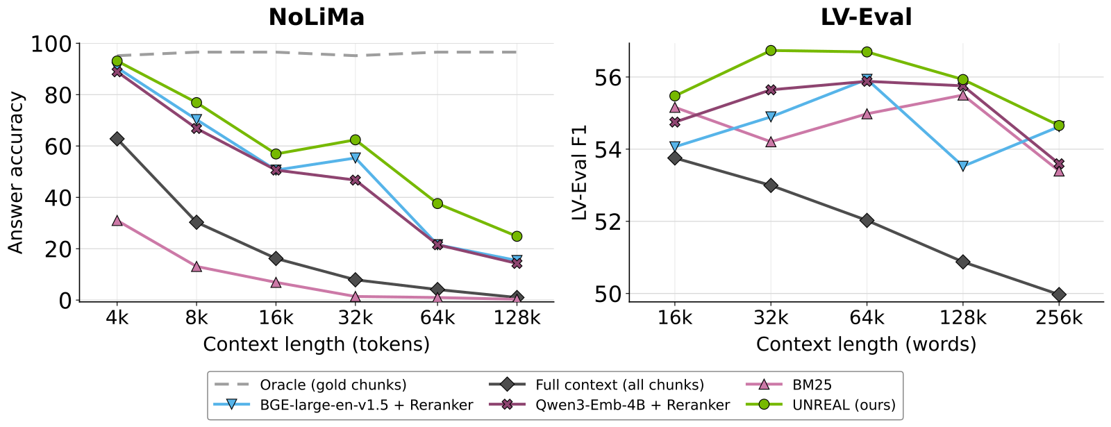
The 1.0% is Nemotron-3-Nano reading the full 128K-token haystack and answering. Three things put that number in context.

NoLiMa is built to be hard for exactly this: the question and the needle share no keywords, so the model has to make a latent association ("lives next to the Semper Opera" answers "who has been to Dresden"). Its own paper evaluates up to 32K for most models, where GPT-4o falls from 99.3% to 69.7% and Llama 3.3 70B to 42.7%. The 64K and 128K points here are an extension.

Nemotron-3-Nano is a small-active-parameter hybrid. Its full-context score is already about 63% at 4K, against an oracle of about 96%, and below 10% by 32K. A 1.0% at 128K is that curve continuing. It is a real measurement of a real model, and a weak reader to compare against.

The fair comparison is on the same chart: two strong external retrievers with a reranker, given the same chunks and the same generator. At 128K they reach about 16% (BGE-large plus reranker) and about 14% (Qwen3-Embedding-4B plus reranker). UNREAL's 24.83% beats them by roughly nine points, which is a solid result for a retriever with no extra model. It is not a 25x improvement.

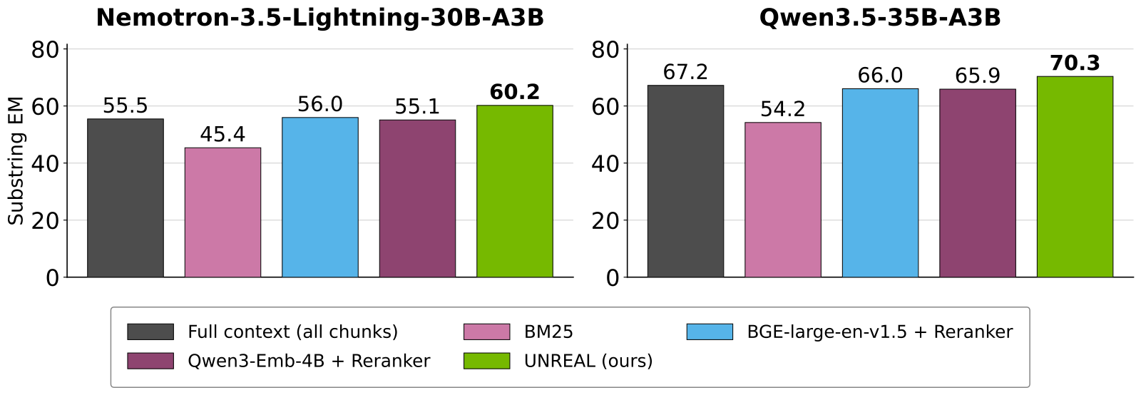
LV-Eval tells the same story more sharply. Full context falls to 49.97 F1 at 256K words; UNREAL reaches 54.66; BGE-large plus reranker sits at about 54.6 on the chart. On HELMET's RAG subset, Qwen3.5-35B-A3B reading the full context (67.2) beats both external retrievers (66.0 and 65.9), and UNREAL edges past it at 70.3. With Nemotron-3.5-Lightning the full context scores 55.5 and UNREAL 60.2.

Two bar charts of substring exact match on HELMET's RAG subset. Nemotron-3.5-Lightning-30B-A3B: full context 55.5, BM25 45.4, BGE-large plus reranker 56.0, Qwen3-Emb-4B plus reranker 55.1, UNREAL 60.2. Qwen3.5-35B-A3B: full context 67.2, BM25 54.2, BGE-large plus reranker 66.0, Qwen3-Emb-4B plus reranker 65.9, UNREAL 70.3. — HELMET's RAG subset, averaged over 8K to 128K. With a strong long-context reader, full context beats both external retrievers and UNREAL wins by about three points (paper, Figure 5).

A few loose ends I could not close from the paper:

Which UNREAL module ran on NoLiMa? The four trained backbones are Qwen3.5-4B, Qwen3.5-35B-A3B, Muse-Glimmer-30B and Nemotron-3.5-Lightning. NoLiMa uses Nemotron-3-Nano, and Section 4 says the long-context modules are "the same ones presented in Section 3". The NVIDIA-Nemotron-3-Nano-30B-A3B config has the same shape as Lightning (2,688 wide, 52 layers), so a Lightning module could be paired with a Nano generator, but the paper does not say so.
Was $n$ chosen on the test set? Figure 6 shows NoLiMa accuracy peaking around twelve chunks and collapsing at both ends. The paper does not say how the $n$ in Figure 4 was picked.
Where does $C_0$ come from in a prompt? The query side needs five BM25 chunks. In the long-context setting they presumably come from BM25 over the prompt's own chunks; the paper does not spell it out. On NoLiMa, which is designed to defeat lexical matching, BM25 scores near zero on its own from 32K up, so at those lengths whatever it adds is not keyword overlap.
Did Muse-Glimmer run past its window? Its config sets max_position_embeddings to 131,072, yet the LOFT-style chart plots its full-context score at 256K and 512K. Part of that collapse may be a model read beyond its trained length.

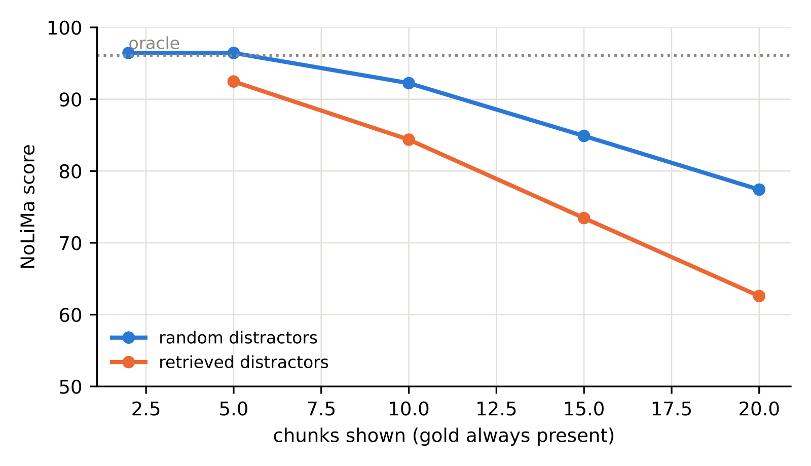
The distractor experiment in the appendix is the best argument for explicit selection. With the gold chunk always present, filling the rest of a 20-chunk prompt with chunks a retriever ranked highly drops NoLiMa to about 62, against about 77 when the filler is random and about 96 for the gold chunk alone. Near-misses hurt more than noise. A model that reads everything is reading all the near-misses.

Line chart of NoLiMa score against chunks shown, from 2 to 20, with the gold chunk always present. Random distractors: about 96 at 2 and 5 chunks, 92 at 10, 85 at 15, 77 at 20. Retrieved distractors: about 92 at 5, 84 at 10, 73 at 15, 62 at 20. Oracle line near 96. — Distractor identity matters: chunks that a retriever ranked highly interfere more than the same number of random ones, and the gap grows with the budget (paper, Figure 11).

Same weights, two pipelines

The toy below lets you poke at the mechanism. Ten invented chunks about a lighthouse keeper, each with two pooled key vectors in a five-dimensional toy space, and a two-hop question. Flip between corpus mode and in-context mode, change $n$ , and turn the BM25 context off. The vectors are made up to show the mechanism. The cost panel is not: it uses the hidden sizes from the configs, the paper's $L_p = 7$ and 21M chunks, and the break-even lengths from the paper's Table 6.

one frozen model, two scales of selectiontoy vectors; the cost panel uses real constants

top-n 2

retrieval input, one forward pass through all layers

BM25 c1BM25 c4What instrument does the lighthouse keeper's sister play?ρ1 … ρ64

read the residual stream at the 64 ρ positions in every full-attention layer, mix the layers with α, pool into groups: here 2 toy query vectors

c1*The lighthouse on Kell Point is kept by Ansel Moore.1.32

c2*Mira Moore, Ansel's sister, plays the cello in the harbour band.1.23

c3The harbour band rehearses on Thursdays.0.42

c4Kell Point's lighthouse was painted red in spring.0.54

c5A ferry crosses to the mainland twice a day.0.00

c6Ansel repairs fishing nets in winter.0.72

c7The bakery on Quay Street sells rye bread.0.00

c8A violin was found in the old customs house.0.73

c9Storms close the ferry for a week each March.0.00

c10The school choir sings at the lighthouse fete.0.65

* the two chunks a complete answer needs. Score = MaxSim over each chunk's 2 pooled key vectors, read once, offline, from the stored index.

second pass: what the generator is given

c1 The lighthouse on Kell Point is kept by Ansel Moore.

c2 Mira Moore, Ansel's sister, plays the cello in the harbour band.

What instrument does the lighthouse keeper's sister play?

complete evidence: both hops are in the prompt

order: by score, as retrieved

trainable: (64 + 1) x 2688 + 6 = 174,726

per chunk: 7 x 2688 in bf16 = 36.8 KB

21M Wikipedia chunks: 790 GB

a 1,024-wide single vector: 43 GB for the same corpus

scored exhaustively, no approximate index

Switch modes and the ranking does not change: same weights, same 64 retrieval tokens, same layer mix, same MaxSim. What changes is where the keys come from and what it costs. Turn BM25 off with top-n at 2 and the violin chunk beats the sister, because the query never learned the keeper's name. That is the toy version of the paper's largest ablation.

The ranking is identical in both modes, and that is the real unification: one set of frozen weights, one set of trained retrieval tokens and layer weights, one layer to read keys from, one scoring rule, one chunk size, trained once. You do not maintain a second model whose embedding space drifts away from your generator's.

What differs is everything around the score:

	corpus index	in-context selection
chunk keys	computed once offline, stored, 7 vectors per chunk	computed per request, each chunk alone, discarded
BM25 context	BM25 index over the corpus	BM25 over the prompt's chunks (my reading)
search	exhaustive MaxSim over all 21M, no ANN	MaxSim over a few hundred to a few thousand
what the generator gets	top $n$ in score order	top $n$ in original document order
KV reuse	none	none: selected text is prefilled again

So there are two code paths, with the same scorer in the middle. That is still a lot less than a RAG stack plus a long-context stack. But "without requiring an external retriever" needs one footnote: the dense retriever is gone, BM25 is not. The paper says as much in its limitations, which mention its reliance on a cheap BM25 initial context.

What it costs

The index

Seven $d$ -wide vectors per chunk is a big index. The paper does not give its size or its precision, so I did the arithmetic, assuming bf16:

Nemotron-3.5-Lightning, $d = 2688$ : 36.8 KB per chunk, about 790 GB for 21M chunks.
Qwen3.5-35B-A3B, $d = 2048$ : about 602 GB.
Muse-Glimmer-30B, $d = 6656$ : 91 KB per chunk, about 1.96 TB.

A single 1,024-wide vector per chunk, BGE-large's size, is about 43 GB for the same corpus. A ColBERT-style index at 128 dimensions per token and about 141 tokens per chunk would be about 758 GB uncompressed, so UNREAL is in the same league as late-interaction retrievers, not embedders (I measured a real one in the pplx-embed-v2-late teardown). And the paper scores every query exhaustively against all 21M chunks: on Nemotron-3.5-Lightning, 4 query vectors times 7 chunk vectors times 21M chunks of 2,688-wide dot products is about 3.2 TFLOPs and a pass over the whole 790 GB index per question. That is fine on a GPU cluster and not how anyone would serve it; there is no corpus-scale query latency in the paper.

The ablation offers a cheaper point. With $L_p = 1$ the Nemotron index drops to one vector per chunk, about 113 GB, and HotpotQA complete-evidence recall@10 goes from 72.93 to 69.11. That is still 20 points above the best baseline, at a seventh of the storage. If I were building this, that is the configuration I would start from.

Building the index is a forward pass over 3B tokens through 42 of 52 layers. With the 2.87B active matrix parameters the paper's Table 6 gives Nemotron-3.5-Lightning, that is roughly $2 \times 2.87\text{B} \times \tfrac{42}{52} \times 3\text{B} \approx 1.4\times10^{19}$ FLOPs by my count, several times what a 335M-parameter embedder would spend. It is a one-off cost.

The long-context pass

For a prompt, UNREAL does more passes but less work per pass. Full context prefills $N$ tokens through all $L$ layers with quadratic attention. UNREAL encodes $N/T$ chunks independently through $\ell_c$ layers (no cross-chunk attention, so linear in $N$ ), runs one pass over $x_{\mathrm{ret}}$ (5 BM25 chunks, the question and 64 retrieval tokens, 910 tokens in their setting), then prefills only $nT$ selected tokens for generation. Appendix C writes the FLOP difference out in full and simplifies it to

\Delta \approx 2\Theta\lambda N + 2 L_a d_a N^2 - 2\Theta\,(nT + |x_{\mathrm{ret}}|)

where $\Theta$ is the active matrix parameters, $\lambda$ the fraction of them above $\ell_c$ , $L_a$ the number of global-attention layers and $d_a$ their width. The first term is the layers UNREAL never runs on the context; the second is the cross-chunk attention it skips; the third is the retrieval pass and the re-encoding it adds. Solving $\Delta = 0$ gives a break-even length. The paper's Table 6 lists 4,117, 6,321 and 13,049 tokens at $n = 5$ for Qwen3.5-35B-A3B, Nemotron-3.5-Lightning and Muse-Glimmer, and 5,569, 8,471 and 17,437 at $n = 10$ . I redid the quadratic from the table's own $\kappa$ and $\lambda$ and got the same numbers within rounding. I also checked $\kappa = \Theta / (L_a d_a)$ against the configs: it implies $d_a \approx 4{,}096$ for all three, and $32 \times 128$ , $16 \times 256$ and $32 \times 128$ are exactly that.

FLOPs are not latency. Measured time-to-first-token on one H100 with vLLM crosses over later.

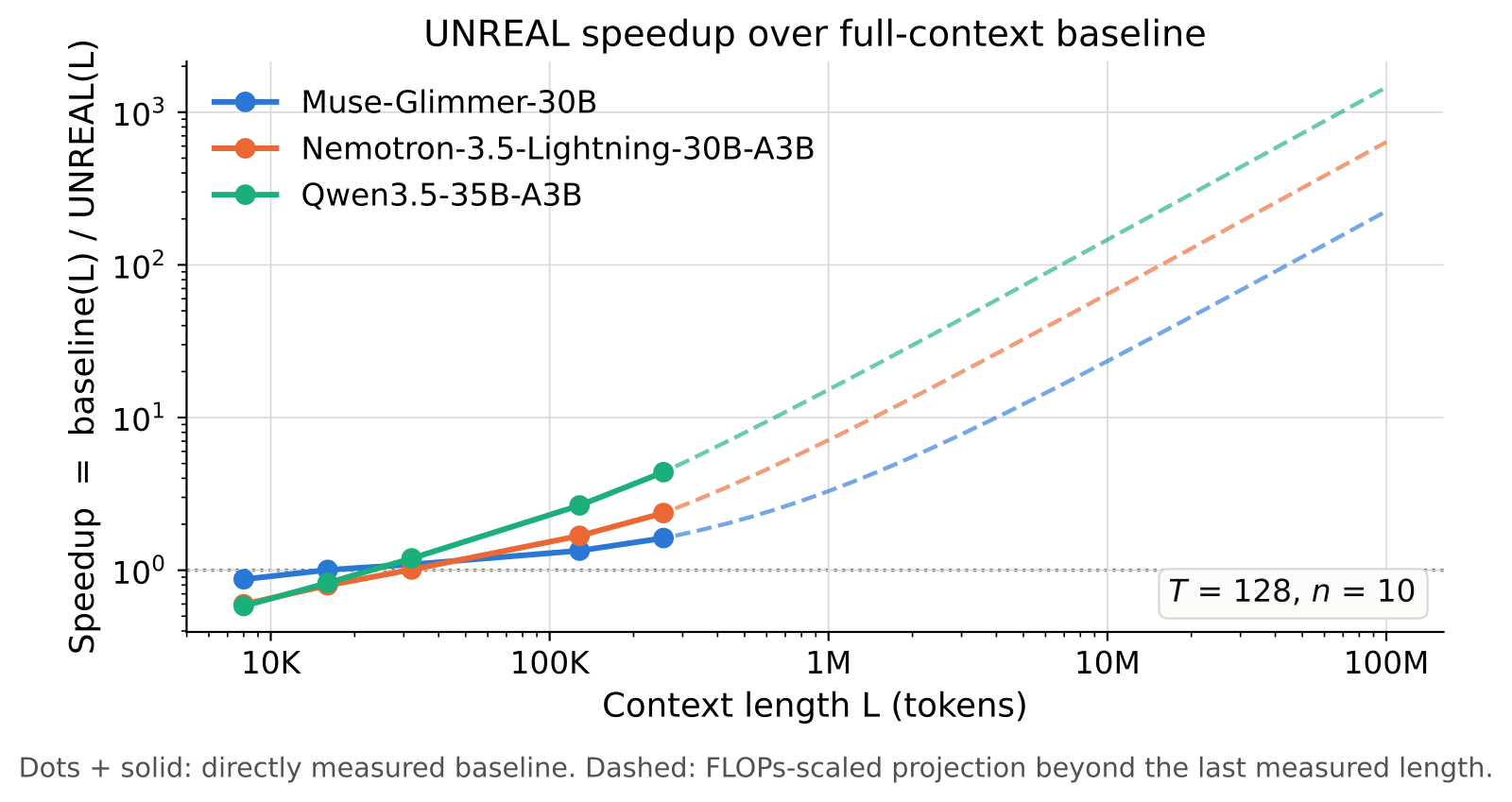
Log-log chart of UNREAL's speedup over full-context inference against context length from 8K to 100M tokens for Muse-Glimmer-30B, Nemotron-3.5-Lightning-30B-A3B and Qwen3.5-35B-A3B, with T=128 and n=10. Solid measured segments run to 256K: at 8K the speedup is about 0.6 for Qwen and Nemotron and about 0.9 for Muse; around 32K all are near 1; at 256K Qwen is about 4.4, Nemotron about 2.4, Muse about 1.65. Dashed FLOP-scaled projections continue to about 1,400, 640 and 225 at 100M. — Time-to-first-token speedup over full-context inference. The solid segment is measured, up to 256K; the dashed segment is the full-context time scaled by the FLOP model. Below about 32K, UNREAL is slower (paper, Figure 7).

Reading the chart: at 8K UNREAL is slower, about 0.6x on the two MoE models. Around 32K it breaks even. At 256K it is about 4.4x faster on Qwen3.5-35B-A3B, 2.4x on Nemotron and 1.65x on Muse-Glimmer, probably because its 39 sliding-window layers already keep its full-context cost down. The big multipliers in the appendix (146x at 10M and 1455x at 100M for Qwen3.5-35B-A3B) are projections: the baseline was only measured to 256K, and everything past that is its measured time scaled by the FLOP model.

The benchmark setup is reasonable, with caveats the paper states itself: random weights and random token ids (it measures speed, not accuracy); chunk-encoding time computed from measured per-chunk throughput rather than timed end to end; the MaxSim step and the orchestration between stages left out. The MaxSim omission is harmless, under 0.01% of FLOPs by their count. The orchestration is not free in a real server, and it is the part I would want measured.

Where it sits among attention-based retrieval

UNREAL is easiest to understand next to the methods it resembles and is not.

Retrieval heads (Wu et al., 2404.15574) showed that a few attention heads do the copying in long-context models; HydraHead builds an architecture around keeping those heads on full attention. UNREAL's untrained baseline in the appendix is in that spirit, per-head keys and queries pooled and dotted, and it is the weak line in Figure 6. UNREAL itself ignores heads entirely.

InfiniRetri (2502.12962) uses the model's attention distribution, training-free, to decide which sentences to carry forward while reading a long input in chunks. That is the closest idea: model-internal evidence selection over a prompt. The difference is that UNREAL trains a read-out for it and reuses that read-out for a corpus.

Quest (2406.10774), RetrievalAttention (2409.10516), MoBA, NSA and MiniMax's sparse attention all select inside attention: per layer, often per head, for every query token, with the whole KV cache still resident somewhere (see SparDA for what offloading it costs). They can change their mind token by token. UNREAL decides once per question, at chunk granularity, before generation starts, and the unselected text simply never reaches the generator. That makes it cheaper and blunter: it cannot go back for a chunk it did not pick, and on evidence-dense work like summarising a whole document it has nothing to offer. The paper scopes itself to sparse-evidence tasks and says so. It cites Quest, MoBA, NSA, InfLLM and Landmark Attention, but not retrieval heads, InfiniRetri or RetrievalAttention.

Against KV compression like KVzip, the trade is similar: KVzip keeps a query-agnostic subset of the cache that works for any next question; UNREAL keeps nothing and re-selects per question. And against agent-managed context in Context Language Models, UNREAL is the single-pass, no-reasoning end of the spectrum, a component an agent could call rather than an agent. The attention field guide has the background on all of the sparse-attention family.

What I would take from it

The idea I would keep is that a frozen generator's residual stream, read with a few hundred thousand trained parameters, is a better retriever for that generator than a separate 4B embedder, at least on Wikipedia-style multi-hop questions with in-domain training. The 4B result shows the effect is not about size. The ablations show where it comes from: a query that sees BM25's first hop, and a read-out that mixes every global-attention layer.

For long prompts, the honest pitch is narrower than the abstract. If your workload is sparse-evidence questions over 32K+ prompts and you already serve one LLM, UNREAL-style selection should beat both full-context reading and an external retriever by a few points, and cost less time-to-first-token from about 32K. It will not turn a 1% model into a 25% model in any sense that matters beyond the chart, because a plain retriever-plus-reranker already gets most of the way.

For a corpus, the index economics are the hard part. The seven-vector index is roughly 790 GB on Nemotron and searched exhaustively; the one-vector variant is about 113 GB and loses under four points. Neither the code nor the trained modules are released, so none of this can be tried yet.

How I checked

I read the arXiv HTML of 2610.08463v1 in full, including all four appendices and every table, and rendered the paper's SVG figures to read values off the charts. Numbers given as "about" are read from charts; numbers given exactly come from the paper's text or tables. I pulled config.json for Qwen/Qwen3.5-35B-A3B, Qwen/Qwen3.5-4B, nvidia/NVIDIA-Nemotron-3.5-Lightning-30B-A3B-BF16, meta-models/Muse-Glimmer-30B and nvidia/NVIDIA-Nemotron-3-Nano-30B-A3B-BF16 from Hugging Face and located the global-attention layers in each. The parameter counts, index sizes, MaxSim cost and index-build FLOPs are my arithmetic from those configs and the paper's constants, with bf16 storage as my assumption. I re-solved the paper's Equation 10 from its Table 6 inputs. NoLiMa's evaluated lengths and its GPT-4o and Llama 3.3 70B numbers are from the NoLiMa paper. I searched GitHub, Hugging Face and the arXiv listing for code or weights and found none; the Hugging Face paper page lists no linked models or datasets. I did not run anything.