2026-10-08 · 23 min · video-generation · diffusion · diffusion-transformers · attention · sparse-attention · fine-tuning
Why read this
Essentialtop 10%Recounts T3-Video's MAC table from code, maps every layer's windows, and finds a duplicated attention pass and a misread theory-vs-practice gap.
- Original, source-checked analysis
- Interactive explanations
- A lasting reference
Image & video generationNeeds datacenter GPUsApache-2.0Practitioner paper
How this was scored
- Is it new?
- 2 of 3: A real new idea, method or capability
- Can I trust it?
- 3 of 3: Reproduces the headline result, or shows from primary files it is wrong
- Can I run it?
- 2 of 3: Open code or weights with real limits
- Will I understand it?
- 3 of 3: Mechanism carried by interactives built from real code or data
- Can I act on it?
- 2 of 3: A concrete recipe, numbers or comparison
- Will it last?
- 2 of 3: A reference for a year or more
- Does it affect many?
- 1 of 3: A specialist community
- Only here?
- 3 of 3: The only place this analysis exists
Score 81 of 100, ranked 14 of 476 rated articles. Each question is answered 0–3 by hand, and a 3 is rare. How articles are scored
A post from @HuggingApps came with a claim I wanted to take apart: "native 4K video, from a 1.3B model. T3-Video retrofits Wan2.1-1.3B with window attention so it generates directly in 3840×2176, no upscaler." The demo zooms into a canyon until single bushes fill the screen.
The Space links three things: the paper, Transform Trained Transformer for Accelerating Native 4K Video Generation
(Jiangning Zhang and eleven co-authors; the README's citation lists ICML 2026), the code at
github.com/zhangzjn/T3-Video, and the weights at
APRIL-AIGC/T3-Video. I read the paper end to end, cloned the code, read the safetensors headers
and pulled the Space's own app.py. My question was simple: a 1.3B model trained at 480p is now being asked to denoise 685,440 tokens per step.
How is that not a week of GPU time?
The answer turns out to be clean and a little surprising. The weights keep their exact shapes. What changes is which tokens each attention call is allowed to see. And once I recomputed the paper's cost table from the code, two things fell out that the paper does not say: one layer in every five runs the same attention twice, and the "gap between theoretical and actual speedup" it apologises for mostly is not there.
- task
- text-to-video
- library
- diffusers
- license
- apache-2.0
- safetensors
- 2 shards
- largest file
- 10.00 GB
- files
- 7
- downloads
- 101
- likes
- 20
repo last modified 2026-10-05
- license
- Apache-2.0
- branch
- main
- tests
- none found
- source
- 2.9 MB
- commit date
- 2026-10-05
by size of tracked source at this commit, file counts in brackets; docs, data and vendored trees excluded
local clone, 2026-10-08 at 09454d4 — branch, commit, commitDate, fileCount, hasTests, languages, license, licenseFile, shallow
shallow clone: counts describe the pinned tree, not the history
Counting the tokens
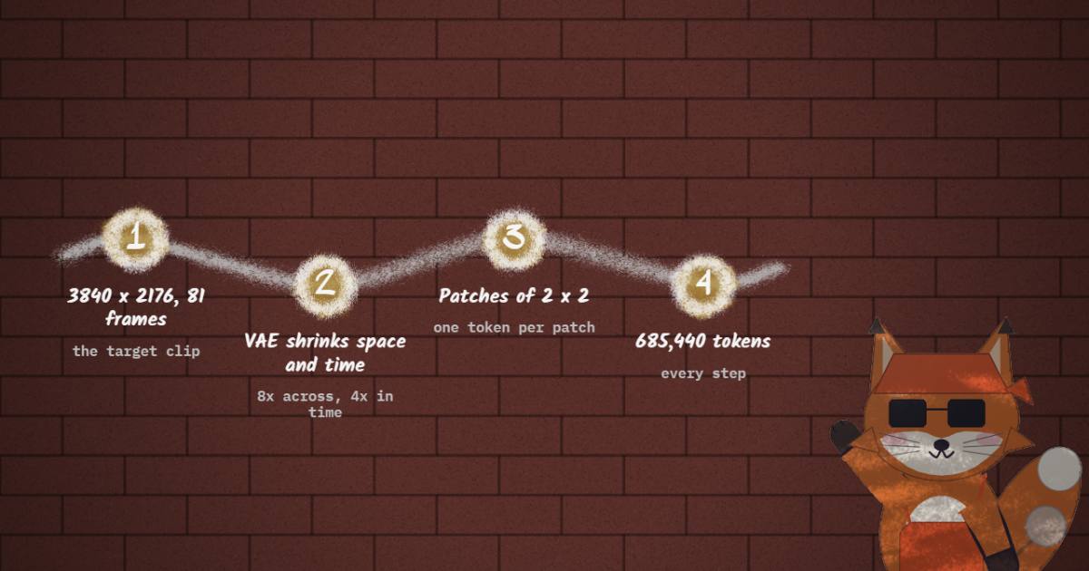
Start with what the transformer actually receives. Wan2.1's VAE compresses 8× in each spatial direction (upsampling_factor = 8,
wan_video_vae.py:1077) and 4× in time while keeping the first frame on its own, so 81 frames become (81 - 1) // 4 + 1 = 21 latent frames
(wan_video_new.py:495). The DiT then patches every 2×2 latent pixels into one token (patch size [1, 2, 2], wan_video_dit.py:640). One token
is a 16×16 pixel square over four frames.
At 3840×2176 that is 240 tokens across, 136 down, 21 deep:
The Space's header says "685k tokens", which is this number. For comparison, the same 81 frames at 832×480 give 32,760 tokens. Going to 4K multiplies the token count by about 21. Full self-attention costs grow with the square of that, so the attention bill goes up roughly 440-fold.
The paper writes the cost of one transformer layer in multiply-accumulates, ignoring biases, with the width and the FFN width:
The first term is the Q, K, V and output projections, the last is the FFN, and the middle one is attention itself: and the
weighted sum over , each . Wan2.1-1.3B has , and 30 layers (wan_video_dit.py:642-649). Plug in
and the attention term alone is 43,299 trillion MACs per forward pass, against 858 trillion for everything else combined.
At 4K, attention is 98% of the model.
Memory is the other wall, and it is subtler than it looks. If you wrote the attention scores out, one layer's 12 heads at bf16 would be bytes, about 11.3 TB. Nobody does that: FlashAttention streams the scores through on-chip memory and never stores them. What you actually hold is activations. One tensor in bf16 is 2.1 GB, and the FFN's hidden state is 12.3 GB. Activations are why the paper reports 59.5 GB to run inference at 4K even with windowed attention, and why the Space had to patch the code to fit a 48 GB budget (more on that below).
Wan2.1's VAE divides each side by 8 and time by 4, and the DiT patches 2 x 2 more, so one token stands for a 16 x 16 pixel square over four frames. At this setting that is 685,440 tokens. Full attention costs 43,299T MACs per forward pass; T3's windows cost 1,007T. The projections and FFN, 857.8T, do not shrink at all, which is why the whole-DiT saving is smaller than the attention saving.
Drag the frame count and switch resolutions and the shape of the problem is plain. The projection and FFN bars move linearly. Full attention moves quadratically and swamps them by 4K. The T3 bar moves linearly too, because its windows stay a fixed size while the video grows.
What happens if you just ask Wan for 4K
Nothing about Wan2.1 stops you from setting height=2176, width=3840. RoPE extends, the convolutions do not care. The paper did it.
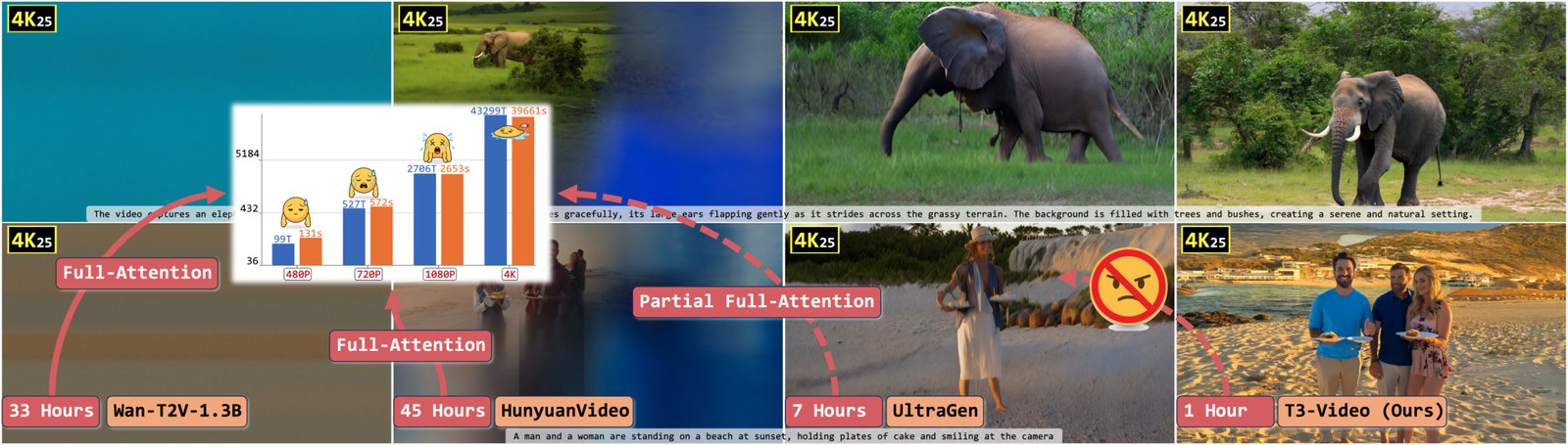
Wan2.1-1.3B at 4K renders a flat teal field. HunyuanVideo smears. Both take a day or more. The model was never trained to place things at these positions, and the attention distribution over 685,440 keys is nothing like the one it saw over 32,760. Brute force is both slow and wrong.
One number in this figure does not match the paper's own table, and I will come back to it: the "33 Hours" label for Wan.
Two windows per query
The obvious fix is window attention: cut the token grid into blocks and let each token attend only within its block. If a block holds tokens, the attention term becomes , linear in . The paper's Figure 2 shows why nobody can stop there. With purely local windows, each block draws its own little scene, and you get a mosaic of disconnected cats. Purely strided windows, where each block takes every n-th token across the whole frame, produce noise.
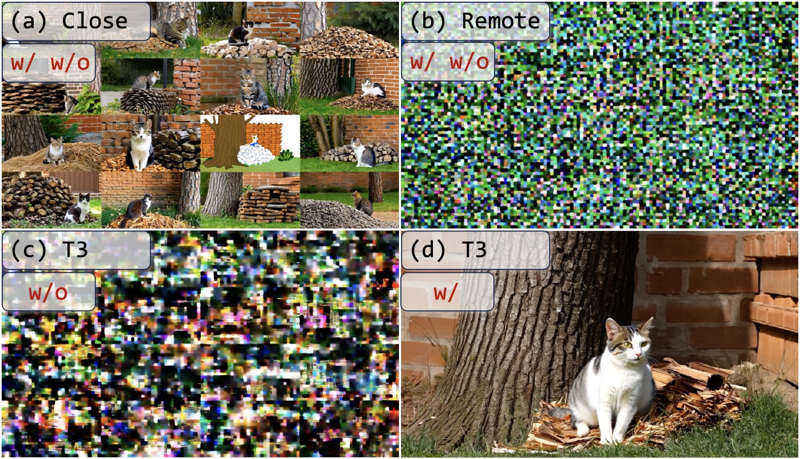
T3's answer is to run both at once and average. In every self-attention layer, each token takes part in two attention calls of the same size. The close call covers a contiguous block around it. The remote call covers a dilated grid: same number of tokens, but sampled every few rows and columns across the entire frame. Both use the layer's existing , , and . Nothing new is added to the model.
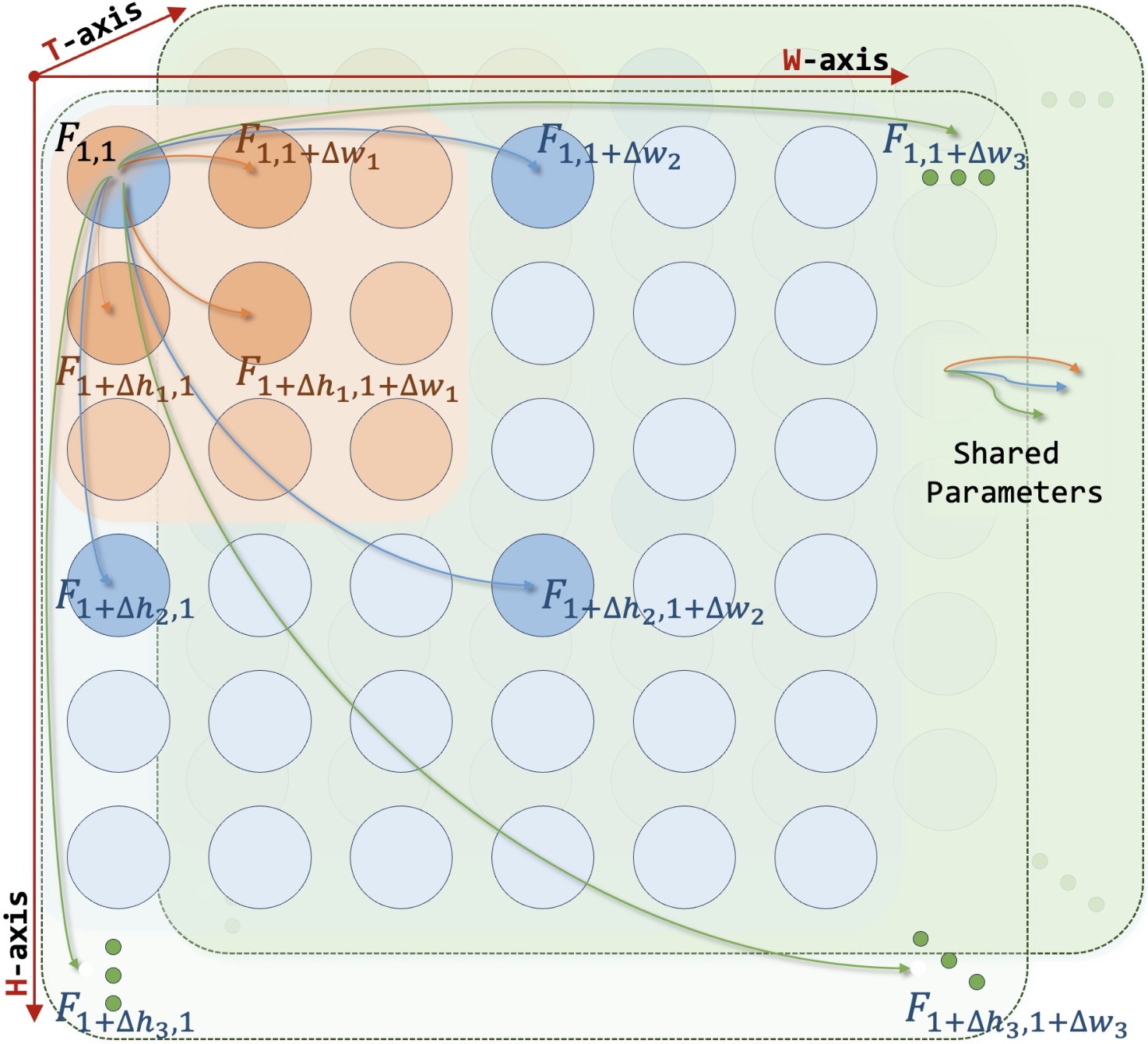
The code is a pair of einops rearranges that differ only in the order of two axes. This is the whole mechanism, from
diffsynth/models/wan_video_dit.py:
q_remote = rearrange(q, 'b (w_t n_t) (w_h n_h) (w_w n_w) d -> (b n_t n_h n_w) (w_t w_h w_w) d', ...)
x_remote = self.attn(q_remote, k_remote, v_remote)
...
q_close = rearrange(q, 'b (n_t w_t) (n_h w_h) (n_w w_w) d -> (b n_t n_h n_w) (w_t w_h w_w) d', ...)
x_close = self.attn(q_close, k_close, v_close)
...
x = (x_remote + x_close) / 2
Read (n_h w_h) as "split the height into n_h blocks of w_h rows" and you get contiguous blocks. Read (w_h n_h) as "take every
n_h-th row" and you get a strided set. Each becomes a batch of short sequences fed to the ordinary flash-attention call. Because the
windows are just a reshape into the batch dimension, the attention kernel itself is untouched, which is what the paper means by a
"one-line" replacement and why it can keep using stock FlashAttention-2.
I like this design. It is cheap to reason about: within one layer every token sees a sparse sample of the whole video through the remote grid, and full-resolution context through the close block. It is the dilated-plus-local trick from image backbones, which the paper credits to its own EMOv2 work, applied without inventing a module.
Five layer types, cycled six times
The paper says the blocking scheme varies by layer, grouped in fives, and leaves the numbers to the code. They are hard-coded in
SelfAttention.__init__ (wan_video_dit.py:199-212), keyed on the layer index modulo 5. (n_t, n_h, n_w) is the number of blocks along each
axis of the 21×136×240 grid:
| layer index mod 5 | blocks (n_t, n_h, n_w) | close window (frames × rows × cols) | in pixels | tokens per window |
|---|---|---|---|---|
| 0 | 21, 1, 1 | 1 × 136 × 240 | one whole frame | 32,640 |
| 1 | 1, 17, 30 | 21 × 8 × 8 | 128 × 128, all frames | 1,344 |
| 2 | 1, 8, 40 | 21 × 17 × 6 | 272 × 96, all frames | 2,142 |
| 3 | 3, 17, 8 | 7 × 8 × 30 | 128 × 480, 7 latent frames | 1,680 |
| 4 | 7, 8, 6 | 3 × 17 × 40 | 272 × 640, 3 latent frames | 2,040 |
Two of the paper's ideas are visible here. The block boundaries move from layer to layer: an 8-row boundary in type 1, 17-row in type 2, 30-column in type 3, so a token cut off from its neighbour by one layer's grid is in the same block in the next. Swin gets the same effect by shifting windows; T3 gets it by changing their shape. And types 1 and 2 span all 21 latent frames while type 0 spans a whole frame, which is the paper's "axis-preserving full attention": every few layers some axis is attended in full. The paper's ablation found that this mix of shapes matters: configurations pushed toward only large or only small ratios scored 67.14 and 68.69 VQA at 720p against 69.37 for the shipped one.
The close branch sees a solid block around the query. The remote branch sees the same number of tokens, one every 17 rows and 30 columns, so it spans the whole frame at low density. Both use the same Q, K and V projections, and their outputs are averaged. Click or drag on the frame to move the query.
Pick a layer type above and click around the frame. In type 1 the close block is a tiny 8×8 square, but the remote set is 64 single tokens spread across the whole 4K frame, 17 rows and 30 columns apart, through all 21 latent frames. The query can see the far corner of the frame, just sparsely.
The layer that does its work twice
Click type 0 in that widget and the remote and close windows coincide. I did not draw it that way for convenience.
With n_t = 21, w_t = 1, and n_h = n_w = 1, the two rearrange patterns (w_t n_t) and (n_t w_t) index the same frames, and
(w_h n_h) with n_h = 1 is the same as (n_h w_h). I reproduced both permutations in NumPy on an index grid of the real shape: for type 0
the two branches gather identical sets of tokens, for types 1 to 4 they do not. So in layers 0, 5, 10, 15, 20 and 25 the model runs
full-frame attention over 32,640 tokens, then runs it again on the same inputs, then averages two identical outputs.
This is not a small inefficiency. Those per-frame windows are by far the largest in the network. Summing over both branches and all 30 layers, I get 1,006.8 trillion MACs of attention per forward pass, exactly the figure in the paper's Table 1, and 82% of it comes from the type 0 layers. Dropping the duplicate branch cuts attention to 594.5 trillion MACs, which takes the reduction against full attention from 43.0× to 72.8×, and the whole DiT forward from 1,864.5 to 1,452.2 trillion MACs, about 22% less. The output would be bit-for-bit the same: the mean of two identical tensors is the tensor.
I have not run this. If the DiT stays compute-bound, as the measurements below suggest it is, a one-line if around the second branch should
take something like a fifth off every 4K generation. The released weights would not need to change.
What was actually trained
A model whose attention pattern changes this much cannot just be loaded and run. Figure 2(c) shows T3 on unchanged Wan weights: noise. So I wanted to know exactly what the released checkpoint is.
The safetensors header of T3-Video-Wan2.1-T2V-1.3B.safetensors lists 825 tensors and 1,418,996,800 parameters, the same names and shapes as
Wan2.1-T2V-1.3B's diffusion_pytorch_model.safetensors, with no LoRA tensors and nothing added. Wan ships in F32; T3 ships in BF16. Paper
Table 1 says the same: 1419.0M parameters for both. This is a full fine-tune of every weight.
I then range-read four matrices from each of the 30 blocks in both files and compared them. Every tensor moved. The relative change averages 6.5% for the self-attention query projection and 5.9% for the key projection, but only 2.9% for the cross-attention query and 2.7% for the FFN output. The training concentrated on the part whose job changed: self-attention moved about twice as far as anything else. The biggest moves are at the ends of the stack, 10.2% for block 0's query and 10.9% for block 28's. I expected the type 0 layers, which keep full spatial attention, to move least. They do not. The layer type makes no visible difference to how far the weights travelled.
The recipe in the paper has three stages:
- Convert Wan2.1 to T3 attention and fully fine-tune at 720×1280 on UltraVideo, 42,184 high-resolution clips with long captions, from which 120 were held out as 4K-VBench. AdamW, learning rate 2e-5, batch size 64, DeepSpeed ZeRO-2, on H20s; the paper says 64 GPUs, against 128 H20s for UltraWan and UltraGen.
- Fully fine-tune that model again at 2176×3840 with 81 frames. The paper says this progressive route converges in 500 iterations; its training-progress figure says results are "satisfactory" by 2,000, and the general training details say 5K iterations. I could not pin down which run produced the released file.
- Optionally, a LoRA (rank 64, learning rate 1e-4) instead of the 4K full fine-tune. It scores slightly lower and is not what is released.
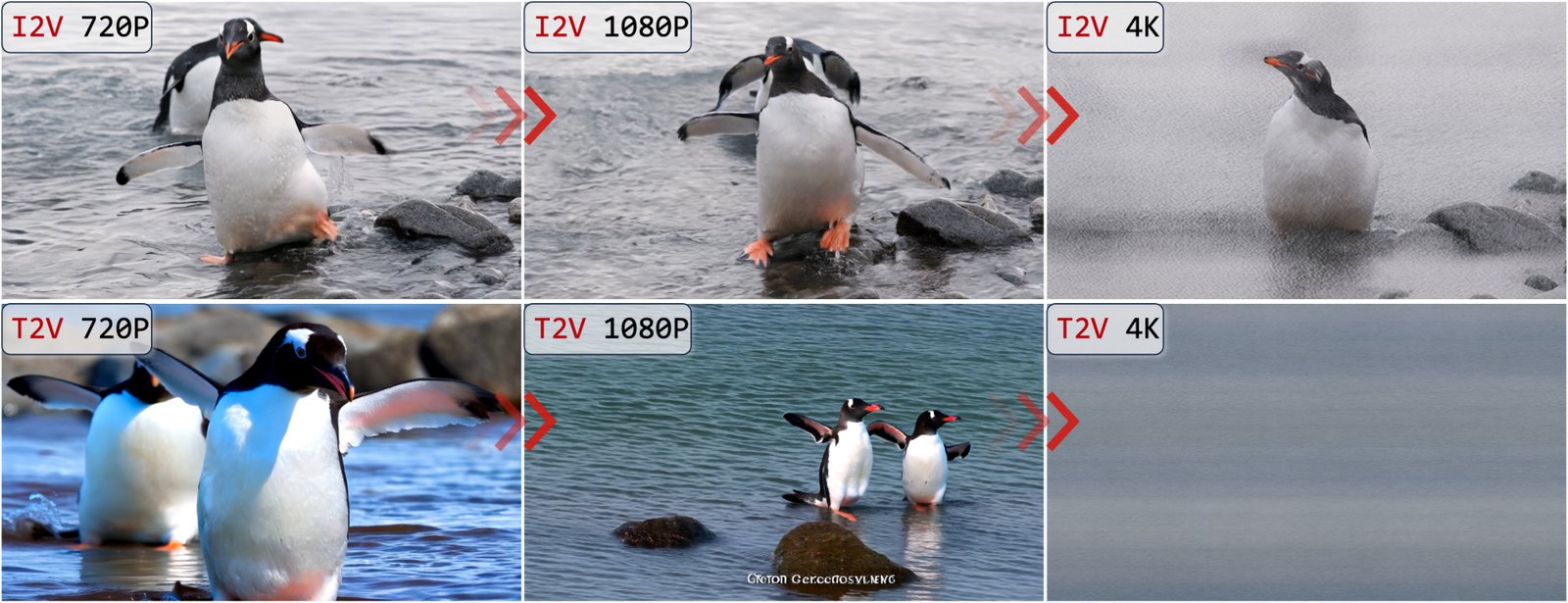
Two figures explain why the stages exist. Fine-tuning at 720p does not transfer to other resolutions for free:
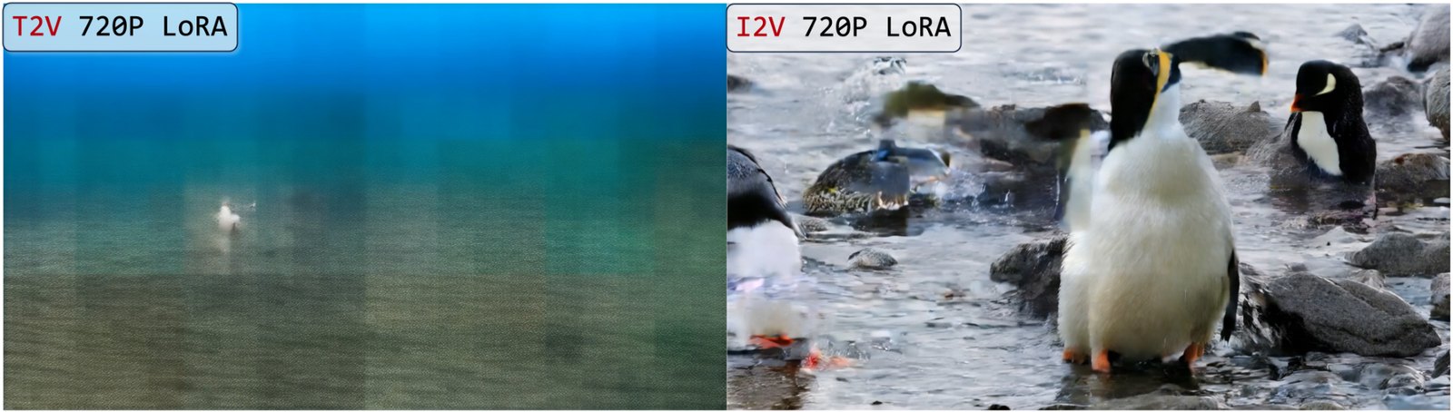
And going straight from Wan's weights to T3 attention with only a LoRA fails, at ranks 32, 64 and 128 alike:
That has a practical consequence. The released window shapes are constants in __init__, the assert self.H % self.n_h == 0 checks enforce
them, and the Space README says the checkpoint "only supports its native training shape: 2176×3840, 81 frames". You cannot ask this model for
a 1080p clip or a vertical video. A different shape means different window constants and, per Figure 5, more fine-tuning. Note also that
2176 is not 2160: the height was picked because 136 divides by 17 and by 8, so you get 16 extra rows to crop.
An hour, not a day
Table 2 is where the paper's speed claims live. It took me a minute to see how its columns fit together. "DiT (50)" is the time for 50 transformer forwards, and the latency column is twice that plus the VAE decoder, because classifier-free guidance runs a conditional and an unconditional pass each step. For T3 at 4K: seconds. For stock Wan2.1 at 4K: seconds. The arithmetic holds in every row.
So on one H20, 50 steps:
- Wan2.1-1.3B at 4K: 79,774.4 s, about 22.2 hours.
- T3-Video at 4K: 4,165.8 s, about 69 minutes, or 37.1 s per transformer forward, 74.3 s per denoising step with guidance.
- The paper's "deployment" variant (8-step DMD2-style distillation with guidance folded in, plus a tiny 9.84M-parameter decoder it calls eVAE): 166.8 s.
The deployment numbers come with a catch. The weights repo holds two files, the T2V-1.3B and T2V-5B DiTs. There is no distilled checkpoint and no eVAE, and the training code is still an unchecked box in the README. The 166.8-second 4K clip is a measurement you cannot reproduce from what is released. At 720p the paper's ablation also shows the distilled model losing about 1.7 VQA points (67.72 against 69.37).
Memory, from Table 3: 59.5 GB at 4K inference, 179.4 GB to train. The Space runs on Hugging Face ZeroGPU and its code comments target a 48 GB
budget. To get there it changes two things in its copy of wan_video_dit.py: RoPE in fp32 instead of the upstream fp64, because "at 685k
tokens the fp64 cast alone allocates >16 GB transients per q/k" (lines 104-107), and the FFN applied in chunks of 65,536 tokens instead of
materialising the 12 GB hidden state at once (lines 374-384). Both are mathematically harmless. It also defaults to 15 denoising steps
instead of the paper's 50, and the X post's own footer reads "15 steps". Its timing constants are labelled in the code as placeholders, so I
would not quote the Space's "10-20 minutes" as a measurement.
The "33 Hours" in Figure 1 is the mismatch I mentioned. Table 2's own components add up to 22.2 hours for the same model at the same resolution on the same GPU. The figure's bar chart uses Table 2's DiT numbers, so I suspect the label came from a different run. Either way the headline survives: one hour against roughly a day.
The speedup gap that is not there
The paper has a paragraph called "Gap between actual and theoretical speed": Table 1 promises 43.0× fewer MACs at 4K and Table 2 delivers only 21.4×, and at 720p it is 30.9× against 4.7×. It blames "software-hardware mismatch" and "reduced compute density from tiling".
But 43.0× and 30.9× are the attention column only. The transformer also spends 857.7 trillion MACs on projections, FFN and cross-attention at 4K, and T3 does not touch any of it. The right theoretical ratio for DiT time is the "All" column: 44,157.1 / 1,864.5 = 23.7× at 4K, and 621.4 / 111.7 = 5.6× at 720p. Measured, the paper gets 21.4× and 4.7×: 90% and 84% of the achievable ratio. Every resolution in the table lands between 84% and 90%.
Put another way, both models run at nearly the same arithmetic rate on the H20. Stock Wan does 88,314 TFLOP per 4K forward in 793.2 s, about 111 TFLOPS. T3 does 3,729 TFLOP in 37.1 s, about 100 TFLOPS. Short windowed attention calls are about 10% less efficient than one giant one. A respectable result, and a more honest framing than the paper's: T3 is close to the limit of what removing attention can buy, and the next win has to come from the FFN, which is now the biggest line item. In the calculator above, toggle "run the per-frame layers once" at 4K and watch the whole-DiT number. The FFN does not move.
What the pixels look like
The claim in the post is about detail at 100%. The X video is a 1440×1080 encode, so it cannot show native 4K pixels in a full frame, but it does switch to a 1440-pixel-wide 100% crop of the 3840-wide output. Below are the full frame and the crop, taken from that video.
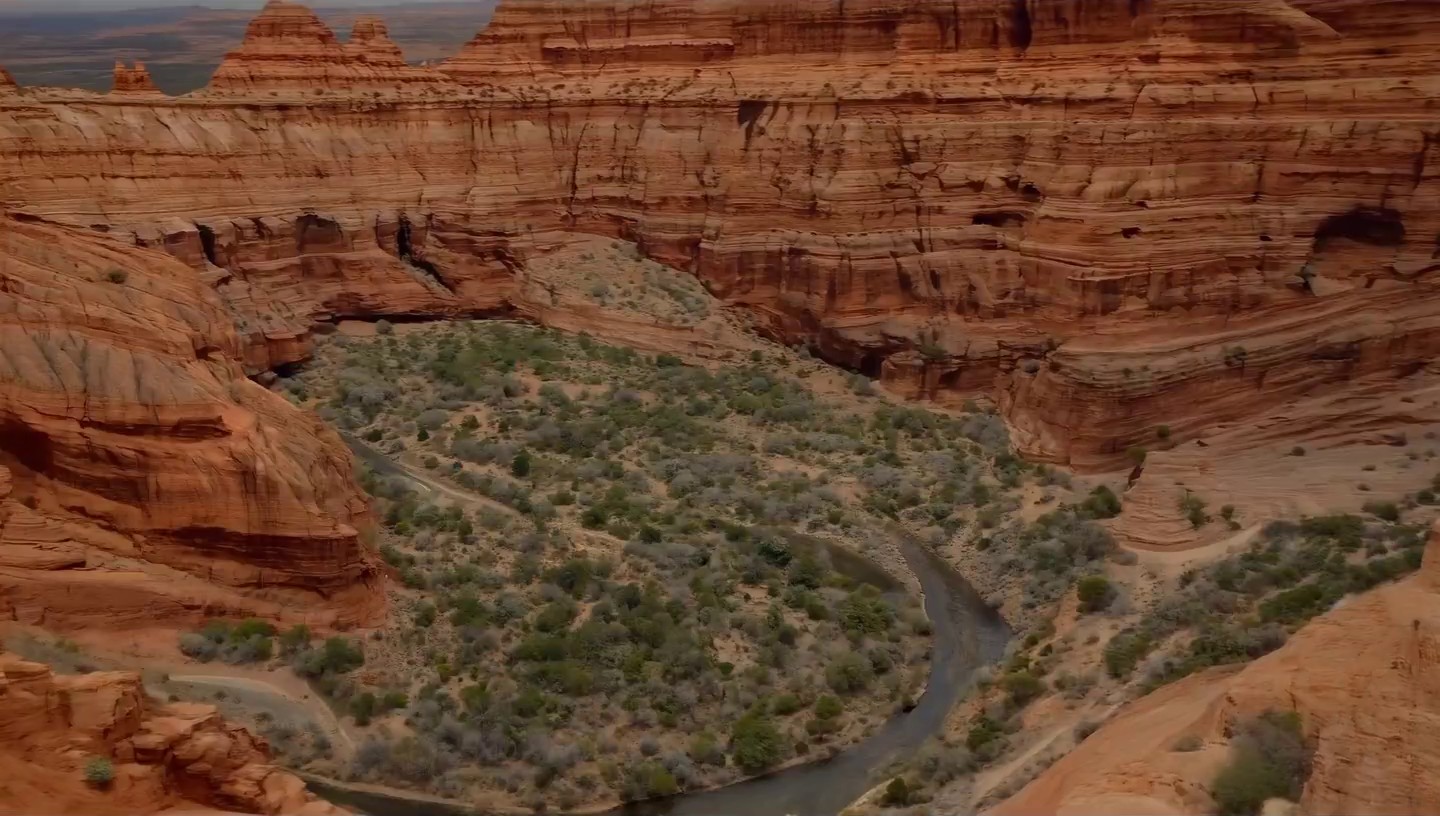
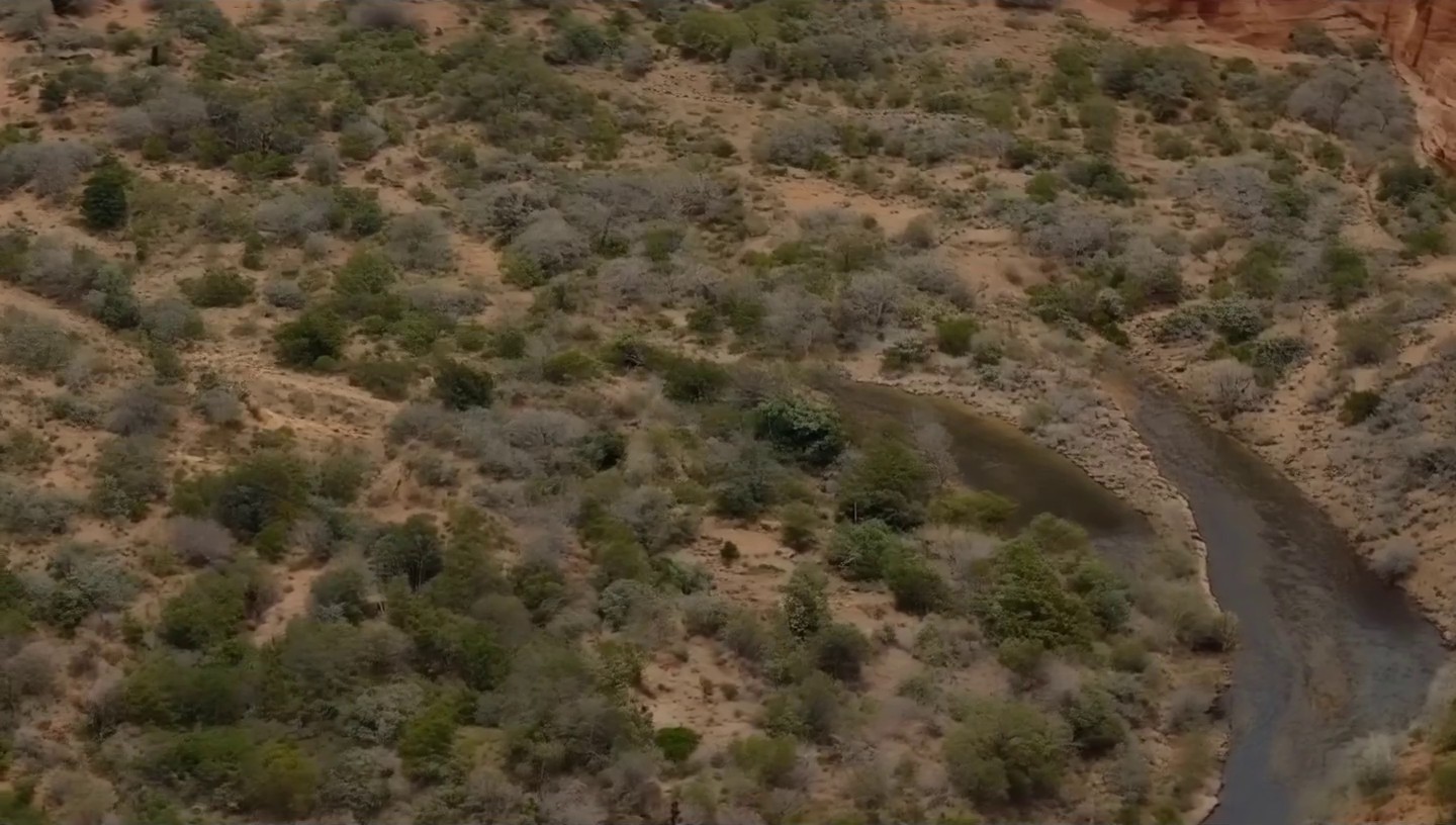
The bushes are individually there, with their own shapes and shadows. They are also soft: no twigs, little texture inside each shrub, and
the edges have the slightly painted look of a diffusion model under-sampled at 15 steps and then compressed by X. It reads as plausible
landscape at 4K, not as photographic 4K. The authors' own teaser frame, which ships in the repo as assets/teaser.jpg at 3812×2160 (so
already resized from 3840), shows the same character up close:
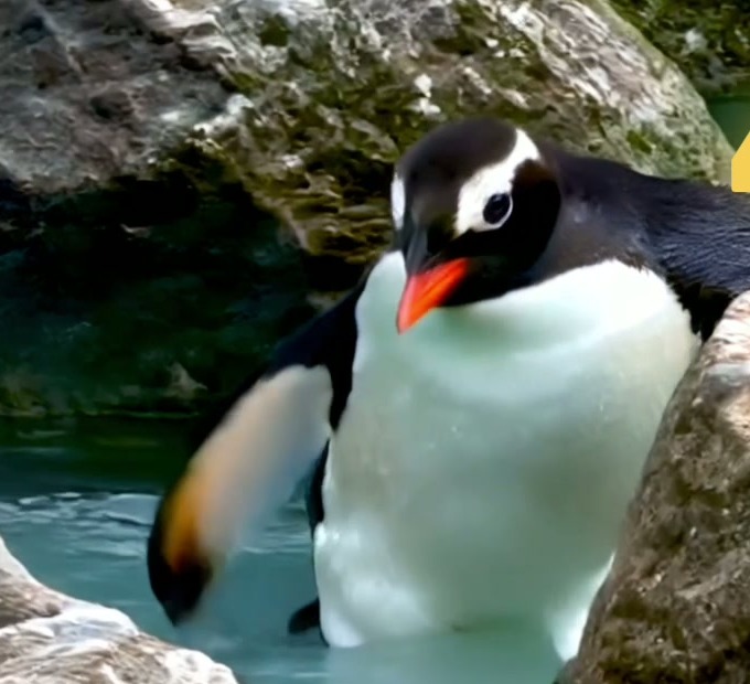
Rock and water texture hold up well. The penguin is clean but smooth, the kind of surface a 1.3B model renders as a gradient. Fine semantic detail at this scale needs capacity, and the paper says as much in its limitations: it did not try Wan2.1-14B for lack of data and compute.
Against upscalers and the other 4K attempts
The standard way to get 4K video is to generate at 720p or 1080p and run a video super-resolution model. The paper's argument against it is that super-resolution invents high-frequency detail that does not belong to the scene and flickers between frames. It is a fair argument, but the paper does not test it. It skips the comparison because UltraGen "already proved superior to cascaded" pipelines, and UltraGen, UltraWan and the UltraVideo dataset all come from overlapping author lists with T3. There is no head-to-head against a current upscaler anywhere in the paper, so the "no upscaler" framing is a design choice rather than a measured win. If I had to ship 4K video tomorrow on a budget, T3 at 720p is 259.9 s per clip on an H20 by the paper's Table 2, and a cascade from there is the obvious baseline someone should run.
The comparisons it does make, on its 120-clip 4K-VBench:
| model (4K) | frames | VQA | VTC |
|---|---|---|---|
| Wan2.1-T2V-1.3B, official | 81 | 30.01 | 0.37 |
| HunyuanVideo, official | 41 | 61.92 | 0.68 |
| UltraGen | 29 | 67.43 | 0.75 |
| T3-Video-T2V-1.3B | 81 | 71.72 | 0.83 |
| T3-Video-T2V-1.3B, LoRA | 81 | 70.78 | 0.79 |
The headline "+4.29 VQA, +0.08 VTC" is T3 minus UltraGen, and the subtraction checks out. VQA is FineVQ, VTC is a text-consistency score from Qwen3-VL-32B. Ten professional raters preferred T3 over UltraGen 71.25% of the time on video quality and 63.42% on detail. Note the frame counts: UltraGen makes 29 frames, T3 makes 81. The "7 hours versus 1 hour" in Figure 1 is UltraGen's 29 frames against T3's 81, which flatters UltraGen if anything.
Against the efficient-attention literature, T3 sits in a particular spot. Sparse methods like Sparse VideoGen, Sliding Tile Attention and Radial Attention try to keep the model untouched and skip work at inference, and VSA trains a learned sparsity pattern. T3 picks a fixed pattern and retrains every weight to live with it. It costs more than the training-free methods and adapts less than learned routing, but the pattern is static, dense inside each window, and runs on stock FlashAttention, which is why its measured speedup tracks its MAC count so closely. The paper also swapped T3 for Swin-style shifted windows under the same training at 720p: 67.34 VQA against 69.37. And at the far end, LinGen's linear-complexity route reportedly cost around 10K H100 GPU-days of training at 512p, which puts the 64-GPU fine-tune here in perspective.
The authors also make a claim I find more interesting than the 4K result: a T3 model can be turned back into full attention and recovers in 500 iterations at 720p (69.51 VQA against the official 70.56). If that generalises, windowed attention becomes a cheap way to pretrain at high resolution and convert at the end. It rests on one table and one model, so I would treat it as a lead, not a finding.
If you have been following this site's video coverage, compare it with SANA-Video 2.0, which goes the other way and makes three of four layers linear, and Sol-Attn and FastH3, which skip attention blocks at inference. The attention field guide puts dilated and local windows in context, and FlashAttention-3 explains why the score matrix never hits memory. LoT Diffusion is the image-side cousin: a DiT whose token granularity varies by region.
Should you use it
If you want native 4K text-to-video from open weights today, this is one of very few options, and the licence is Apache-2.0 on top of Wan2.1's terms. Budget an hour of a 60 GB-class GPU per 50-step clip, or follow the Space and accept 15 steps and softer detail. You get one shape, 2176×3840 at 81 frames, and nothing else without retraining.
The idea is worth more than the checkpoint. Two windowed passes with shared weights, cycled through a few shapes, is a small, portable change you can apply to any DiT you are willing to fine-tune. If you do, run the per-frame layers once.
How I checked
- Read the paper (arXiv 2512.13492v2, HTML) in full, the repo at commit
09454d4, and the Space'sapp.py,README.mdand its modifiedwan_video_dit.py. Code quotes carry file and line. - Read both safetensors headers by HTTP range request: tensor names, shapes, dtypes and parameter counts. Then range-read the self-attention Q and K, cross-attention Q and FFN output matrices of all 30 blocks from both files and computed the relative change. Nothing else was downloaded and no model was run.
- Rebuilt the close and remote window permutations in NumPy on an index grid of shape 21×136×240 to confirm which layer types give identical windows, and recomputed Table 1's attention, projection and FFN MACs from the config. Every 4K figure matched to the printed decimal.
- Recombined Table 2's columns to confirm latency = 2 × DiT + decoder in every row, and divided Table 1 MACs by Table 2 times for the throughput estimates. Those are my numbers, from the paper's.
- The 100% crops are frames from the 1440×1080 video in the X post and a crop of the repo's teaser image. Neither is a raw output file; I could not run the Space myself.
- Not checked: the deployment variant (weights not released), UltraGen's timing, the human study, and which training run produced the released checkpoint.