2026-10-06 · 29 min · algorithms · theory · math · formal-methods · attention
Why read this
Notabletop 60%The 3SUM/APSP refutation from reduction chain to leaf count, with the identity checked exactly, the practicality arithmetic, and which lower bounds survive.
- Genuinely new idea
- Original analysis
- A lasting reference
Agents & harnessesNothing to runResearch paper
How this was scored
- Is it new?
- 3 of 3: Changes how the field does something
- Can I trust it?
- 2 of 3: Measures key facts from files, code or configs
- Can I run it?
- 0 of 3: Closed, nothing to run
- Will I understand it?
- 2 of 3: Mechanism from first principles with figures
- Can I act on it?
- 1 of 3: General advice
- Will it last?
- 2 of 3: A reference for a year or more
- Does it affect many?
- 1 of 3: A specialist community
- Only here?
- 2 of 3: A teardown or measurement few others did
Score 58 of 100, ranked 256 of 445 rated articles. Each question is answered 0–3 by hand, and a 3 is rare. How articles are scored
Satyajit sent me this paper with one line: "is this real?" I opened it expecting the usual fine print. A restricted model of computation, perhaps, or a randomized algorithm for a special input distribution, or a log factor dressed up as a breakthrough. It is none of those. Josh Alman (Columbia) and Virginia Vassilevska Williams (MIT) give a deterministic algorithm for 3SUM on integers of polynomial size in time, and one for all-pairs shortest paths (APSP) on directed graphs with polynomially bounded integer weights in time (arXiv 2610.06783, posted 5 October 2026). Both beat the textbook algorithm by a polynomial factor, which is exactly what the 3SUM hypothesis and the APSP hypothesis said could not happen.
The second surprise is in the abstract itself: "Claude, an AI model developed by Anthropic, discovered the algorithm that refutes the 3SUM, APSP, and Exact Triangle hypotheses." The authors then simplified it, extended it and wrote it up, and they say they take full responsibility for the paper.
The exponents look like a rounding error. They are not, and the reason is the most interesting part of the story. The new idea lives entirely in one lemma about thin matrix products. Everything else is plumbing the field built over fifteen years to prove that problems were hard, now run backwards as algorithms. I read the paper end to end, checked the central identity exactly, ran the recursion at toy scale, and redid the exponent arithmetic. This page is what I found.
What the field bet on
Fine-grained complexity is the part of theory that asks not "is this polynomial?" but "which polynomial?". It cannot prove that 3SUM needs time (nobody can prove super-linear lower bounds for anything in this regime), so it does the next best thing. It picks a few problems whose obvious algorithms have resisted decades of attack, assumes they are optimal, and then proves, by reduction, that a long list of other problems inherit that hardness. The paper names three such pillars:
- 3SUM: given integers in , are there three that sum to zero? The hypothesis says time on a word RAM.
- APSP: shortest-path distances between all pairs in an -vertex weighted graph. The hypothesis says for polynomially bounded integer weights.
- SETH: CNF-SAT on variables needs time. Through Orthogonal Vectors it gives quadratic lower bounds for edit distance, LCS and, closer to this site, attention.
The 3SUM algorithm is the one everyone writes in an interview. Sort, fix the smallest element, walk two pointers inward:
// three-sum.ts: the O(n^2) baseline the hypothesis said was optimal
export function threeSum(a: number[]): [number, number, number] | null {
  const s = [...a].sort((x, y) => x - y)
  for (let i = 0; i < s.length - 2; i++) {
    let lo = i + 1
    let hi = s.length - 1
    while (lo < hi) {
      const t = s[i] + s[lo] + s[hi]
      if (t === 0) return [s[i], s[lo], s[hi]]
      if (t < 0) lo++
      else hi--
    }
  }
  return null
}
For APSP the cleanest baseline is the product, , which is matrix multiplication with replaced by and by . APSP and the product have the same complexity up to constant factors, a classic result the paper cites from Fischer–Meyer and Aho–Hopcroft–Ullman. Squaring the weight matrix times gives all distances:
# apsp.py: the cubic baseline, via repeated (min,+) squaring
INF = float("inf")

def min_plus(A, B):
    n = len(A)
    return [[min(A[i][k] + B[k][j] for k in range(n)) for j in range(n)] for i in range(n)]

def apsp_by_squaring(W):
    # W[i][i] = 0, W[i][j] = INF when there is no edge; no negative cycles
    n, D, steps = len(W), W, 1
    while steps < n - 1:
        D, steps = min_plus(D, D), steps * 2
    return D
Both snippets run as written (I ran them on small inputs). The reason nobody could beat them is that the usual weapon for "multiply faster", Strassen-style algebra, needs subtraction, and has no inverse. Fast matrix multiplication does not apply to the semiring.
-25 + -10 + 10 = -25 → too small, move lo right
found so far: none
- n² operations
- 10^18
- n^1.999125
- 10^17.99
- speedup from the exponent
- 1.018x (below 2x until n ≈ 10^344)
A billion numbers (n = 10^9) gets a 1.8% exponent dividend, before the algorithm pays any of its constants. The hypothesis was never a claim about practical sizes; it said the exponent 2 could not move at all, and it moved by 0.000875.
The history is a long list of shaved logarithms, which is why the hypotheses felt safe. For 3SUM, Gajentaan and Overmars (1995) showed a family of geometry problems (three collinear points, minimum-area triangle, motion planning) are all at least as hard as 3SUM, and named the class. Baran, Demaine and Pătraşcu (2008) got integer 3SUM below by about factors using word-level parallelism. Then in 2014 Grønlund and Pettie posted a paper whose abstract literally says "we refute the 3SUM conjecture" (arXiv 1404.0799): they showed 3SUM has decision trees of depth and gave a real algorithm in time. That refuted the original, stronger form of the conjecture (that was exactly right) and the field restated it as , which survived. Chan's 2020 algorithm pushed the saving to about for real inputs, and Kane, Lovett and Moran showed that linear decision trees need only queries for -SUM (arXiv 1705.01720). So the information needed was always nearly linear. Nobody could turn it into time.
APSP followed the same pattern. Fredman's 1976 trick gave -depth decision trees and a saving. Forty years of polylog improvements later, Ryan Williams's 2014 algorithm (arXiv 1312.6680) reached using circuit complexity and Coppersmith's rectangular matrix multiplication. That was faster than any polylog shave and still slower than for every . Before this paper it was the fastest known APSP algorithm.
What made these hypotheses load-bearing was the reductions built on them. Vassilevska Williams and Williams (FOCS 2010) proved that APSP, the product, Negative Triangle, Second Shortest Path, Replacement Paths and more are subcubic-equivalent: one falls only if all fall. Pătraşcu (STOC 2010) connected 3SUM to set disjointness and through it to dynamic data structures. By 2026 there were dozens of " requires unless 3SUM is false" results across geometry, strings, graph algorithms and dynamic data structures, and the APSP class had grown to Radius, Median, Tree Edit Distance and Maximum Subarray. One fact about reductions was always sitting there in plain sight. The paper puts it better than I can: "a reduction from to , proved in order to show that is hard, is also an algorithm for whenever turns out to be easy."
Following the chain down
The paper's Figure 8 is the whole proof architecture on one page, and it reads best from the bottom up.
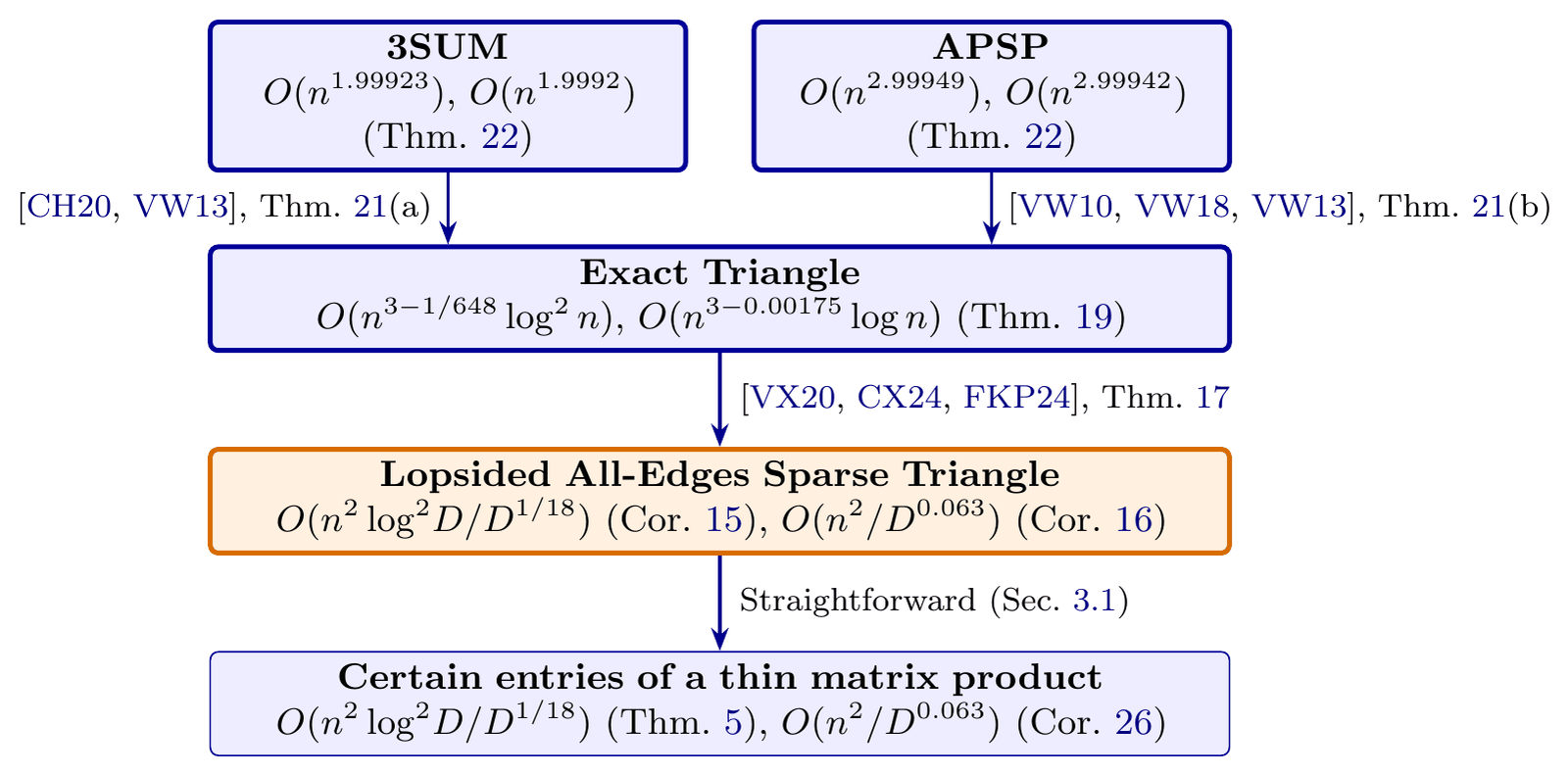
Exact Triangle sits in the middle. You get a complete tripartite graph on parts of vertices each, with an integer weight on every edge, and ask whether some triangle has weights summing to zero. 3SUM reduces to it deterministically: instances on vertices per part (Chan–He and Vassilevska Williams–Williams). So does the product: an Exact Triangle algorithm running in on vertices gives in . Those two reductions are old and the paper cites them unchanged.
Below it sits Lopsided All-Edges Sparse Triangle, and this is where the paper does its own reduction work. Take a tripartite graph with two big parts and of vertices and a small middle part of at most vertices, edges anywhere between and the big parts, and a set of query pairs . For each query pair, decide whether and have a common neighbour in . Write the two biadjacency matrices as and , and the question becomes: compute for every . A thin matrix product, of which you want only a sparse set of entries.
The reduction from Exact Triangle to that problem (Theorem 17) is short enough to sketch. Pick a prime and reduce every weight mod . Group the pairs by their residue . For a group and a piece of , build a middle part whose vertices are pairs with , and connect
A query pair then has a common neighbour exactly when some makes the triangle's weight . Every true zero triangle is caught; hashing also lets in false positives, which a scan of the piece weeds out afterwards. The prime is chosen deterministically, by counting each candidate's false positives with a polynomial-matrix product and keeping the one with the fewest, a trick the paper borrows from Fischer, Kaliciak and Polak's deterministic 3SUM-hardness work. Earlier versions of this reduction were randomized; this one is not, which is why the headline algorithms are deterministic.
The exponent bookkeeping explains why the final numbers are so small. With , each lopsided instance costs instead of , and there are about instances. The witness scans cost . Balancing gives , and the Exact Triangle time is . Each step up the chain then loses more:
So 3SUM lands at and APSP at , which the paper rounds up to and states as in Theorem 22 (the abstract's is the bound from the simpler Theorem 5 path, ). The reduction from Exact Triangle keeps half the saving, and 3SUM and APSP keep a half and a third of what is left. The authors say plainly in their conclusion that these reductions were "designed to prove hardness, where it only matters that they keep some polynomial saving", and that using them as algorithms is now a research problem of its own. Their footnote 10 already notes cheaper routes they chose not to write up.
Why a thin product looked untouchable
Before the new algorithm, there were two ways to get entries of with of size and of size :
- Compute each wanted entry as an inner product: operations.
- Compute all of with fast rectangular multiplication: for , that is , which is optimal for writing down numbers.
The reductions produce wanted entries. Option 1 costs ; option 2 costs . The paper's Theorem 1 does better than both:
It spends polynomially less than one operation per entry of the full product. In graph language the balanced version of this problem has a well-known algorithm (Alon, Yuster and Zwick), which is even if ; on the graphs the reductions produce, vertices of degree about , that equals the brute-force . Matrix multiplication is a tool for dense outputs; this instance asks for a sparse output of a dense product, and there seemed to be no way to exploit that. The trick is to look inside a fast matrix multiplication algorithm and notice that most of its work only feeds entries you did not ask for.
Ten multiplications for thirteen
Strassen's algorithm multiplies matrices with seven products instead of eight and recurses. The multiplications all happen at the leaves of a recursion tree; the additions on the way down ("encoding", from alone and from alone) and on the way up ("decoding") are cheap. The new algorithm keeps that shape but swaps Strassen's identity for one Schönhage published in 1981, which computes two unrelated products at once:
- an outer product of and : nine numbers ;
- an inner product of and : one number.
Separately that is multiplications. Schönhage does it in ten. Extend the 's to a matrix whose columns sum to zero, and the 's to whose rows sum to zero:
The ten products are for , plus . Output reads alone. Output is the sum of all ten. Expand : the terms cancel against ; the cross terms and sum to zero because of how and were padded; what remains is , the inner product, exactly. The nine are plus an error
and every term of pairs an outer output with at least one inner input. Schönhage stated this as a border-rank identity with an that goes to zero; the paper sets and argues the error away combinatorially instead.
The x·y cross terms cancel against P0, and the p·y and x·q terms cancel because the columns of p̂ and the rows of q̂ sum to zero.
| 128/28 | -18/-21 | -42/-35 |
| -5/-4 | 7/3 | 8/5 |
| -52/-16 | -18/12 | 20/20 |
got / x_i·y_j. Shaded cells carry the error E, which always contains a p or a q.
With p and q zeroed every z_ij is exact. That is the whole reason the error is harmless in the recursion: an entry the algorithm reads off a z_ij level only ever sees outer inputs there.
I did not want to take Lemma 6 on trust, so I wrote the ten linear forms down as coefficient tables and expanded the identity symbolically, monomial by monomial. The left-hand side and agree on all 33 nonzero monomials, every coefficient is , and the widget above evaluates the same forms on random integers. Two structural facts matter later, and both are visible in the widget: only feeds , and every term feeds .
Recursing on strings
Apply the identity at levels and you get a tree with leaves, one per string of terms. Each level independently picks "outer" or "inner", so one run computes different matrix products at once. Restrict to the products that pick "inner" at exactly levels. Each of those multiplies a matrix by a one, and there are of them, all completely independent: you can feed any pairs of matrices into one run (Lemma 9). The error never reaches those outputs, because an term needs an inner input at a level where the output is outer, which would give the input string more than inner levels, and such inputs are set to zero.
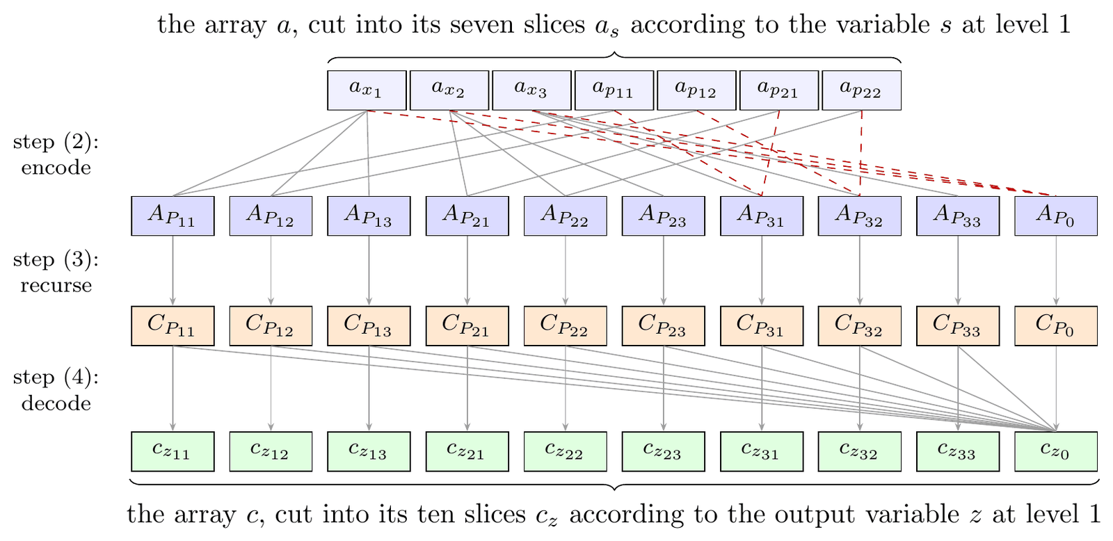
I implemented that recursion directly in Python (a dictionary per array, no tricks) and fed it random matrices: for ; ; and , every one of the 243, 2,916 and 486 checked output entries equals the true . Tiny, but it confirms that the indexing in Section 2.3 means what I think it means.
To multiply a big by , the paper cuts into row blocks of rows and into column blocks, groups blocks into a band, and treats a row band times a column band (a "tile") as one run of the recursion. With fixed by the problem, is the knob. The paper sets . Computing the whole product that way would be wasteful (about operations; is the efficient choice for full products). The reason for 19 shows up in the next step.
The new idea: visit only the leaves you need
Two changes turn the full multiplication into the sparse one.
The first change shares the encodings. The number multiplied at leaf is , where depends only on the left input array and only on the right. A row band takes part in many tiles, so its encoded numbers are computed once and reused. The condition exists mostly to make this one-off cost negligible.
The second prunes the recursion. Each call receives the set of output strings wanted from it and only
recurses into children that feed one of them. The algorithm, Pruned, visits exactly the leaves that
contribute to some wanted entry, each once, however many entries share it (Lemma 10). So the running
time is the size of the union of the wanted entries' leaf sets, not the sum.
The sum alone would be a disaster. One output entry, with inner set of size , is fed by leaves: at its inner levels a leaf may pick any of the ten terms, while at the other levels it must pick the one matching the entry's . , worse than computing the inner product directly with multiplications. The whole argument is about how much those leaf sets overlap.
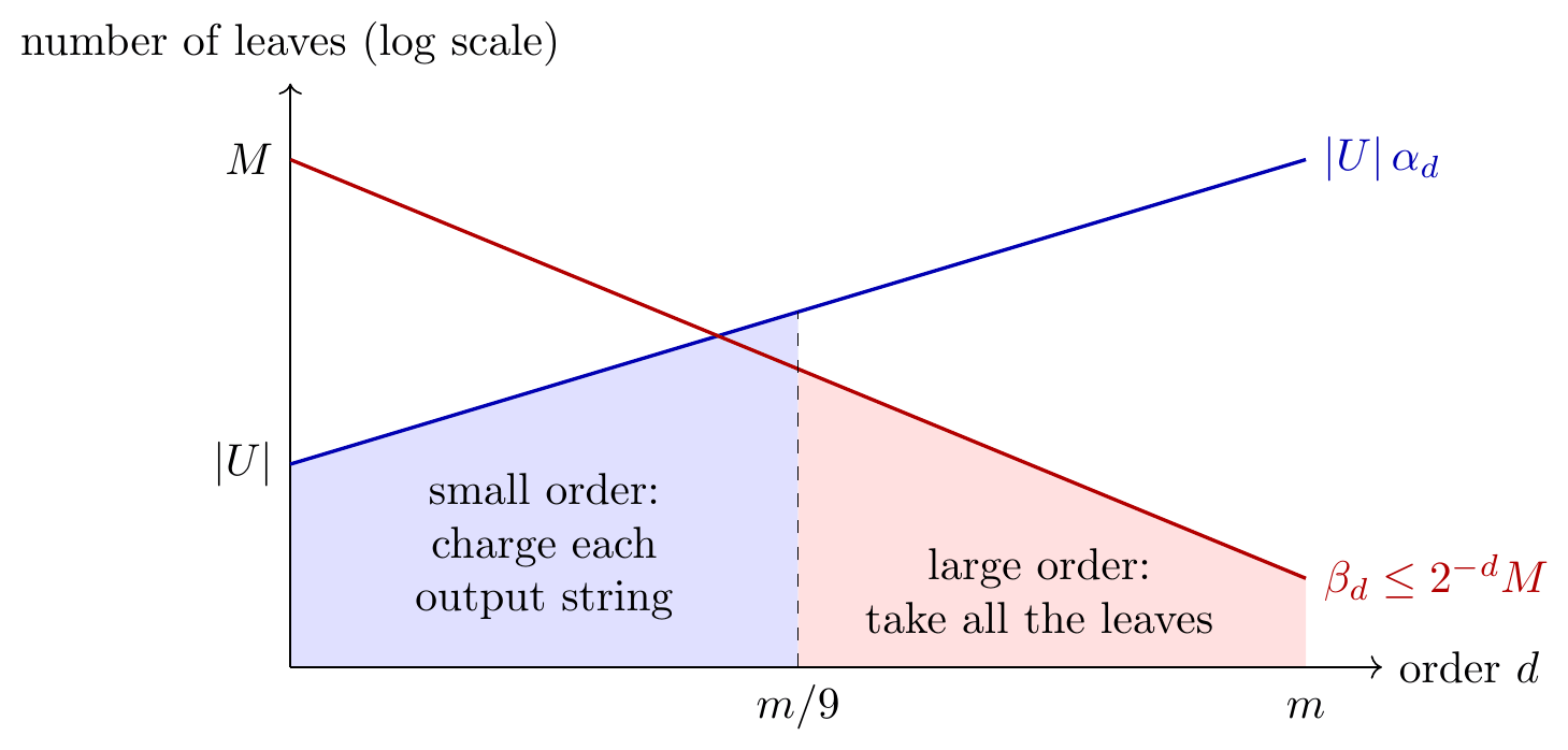
The paper classifies leaves by order: minus the number of levels at which the leaf picks . The order-0 leaf of an output entry picks at all its inner levels. It is the entry's private leaf, and no other entry uses it. A leaf of order swaps for one of the nine at of those levels, and because also serves the outer product, that leaf is shared by every output entry whose inner set contains the leaf's remaining levels.
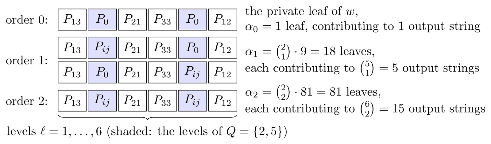
Two counts carry the proof:
, the number of output entries in a tile (one private leaf each). For ,
so the total number of order- leaves halves with every step in . There lies the reason for : at , the ratio is close to 1 for small and the high-order leaves are as numerous as the entries themselves.
Now bound the union for a wanted set two ways at each order and take the smaller: charge each wanted entry for its own order- leaves (), or just take every order- leaf that exists (). For small orders the first is smaller, for large orders the second. Splitting at ,
where the small-order side uses the inequality (it comes to 207.83; I checked). With , that is leaves for the tile's wanted entries: fewer than one per entry of the tile, and far below the of the inner-product route. Paying per leaf for the bookkeeping gives Theorem 5, .
- entries in a tile, M
- 10^169.0
- wanted, |U| = M/√D
- 10^166.3
- inner products one by one, |U|·D
- 10^171.7
- each entry's leaves separately, |U|·10^m
- 10^175.3
- bound on leaves visited, Σ min
- 10^168.7 2.01x fewer than M
At L = 19m the red bars halve (or better) at every step, so the large orders cost almost nothing and the bound lands below M by about D^(1/18), which is 2x at m = 9. Push L down toward 10m and the red bars stop shrinking: the saving disappears. Increase m and the saving grows, while the matrix the tile has to fit inside grows as D^18.
The widget computes those two bounds from the paper's formulas, in log space, for any and any ratio . At and () the bound lands 2.01 times below , right on the paper's . Slide the ratio down to and the bound rises above for every : the pruning buys nothing. It is the clearest demonstration I know of why the exponent 18 is in the theorem.
The data-structure version in Section 4 reuses this split. Preprocessing adds up the high-order leaves into "boxes" ahead of time; a query for one entry, not known in advance, reads its few low-order leaves plus a few boxes. With and switching order , preprocessing costs and each query (Corollary 26), which improves the saving from to and is where the headline exponents come from. The authors say they derived this version themselves, along with its consequences for hinted Online Matrix-Vector multiplication. The theoretical ceiling of the technique is , set by the identity : at a tile has as many outputs as the recursion has leaves.
Why Schönhage and not the identities behind today's best ? Footnote 4 is candid: "prior to this work, the authors had tried approaches like this using the Coppersmith–Winograd identities [CW90] and more, without success." The argument depends on two properties of Schönhage's tiny identity: each is fed by a single term, and every coefficient is . Those are precisely the details that tensor-rank language abstracts away, which may be part of why nobody looked.
How small is 0.0008?
Smaller than any input you will ever have. I worked the numbers out because "galactic" gets used loosely.
The speedup the exponent buys for 3SUM is . For a billion numbers that is 1.018, a 1.8% improvement, with every constant set to 1. To be twice as fast as on exponent alone, you need , about . For APSP the saving is and the 2x point is , about . There are roughly atoms in the observable universe.
The constants are not 1, and they are where the real cost hides:
- Theorem 5 needs . Even the smallest legal case, (), needs , and its saving is 1.08, which the factor eats immediately.
- The encodings are enormous. At , and every band's encoding has numbers. A saving of 2x from needs , and encodings of numbers.
- The proof of Corollary 26's bound checks its inequalities only for , that is , and treats smaller as "bounded by a constant". Through the Exact Triangle reduction that means before the improved machinery is doing anything.
The authors do not pretend otherwise: "The new algorithms are algebraic and potentially impractical in their current form: the constants hidden in the are enormous, and the exponents can likely be improved." If you run 3SUM or shortest paths in production, nothing changes for you. If you write a paper that says " needs time unless 3SUM is false", a lot changes.
What falls, what loses its evidence, what stands
3SUM → n^(1/2) Exact Triangle instances of n^(1/2) vertices [CH20, VW13] → lopsided triangles.
now: O(n^1.9992), deterministic
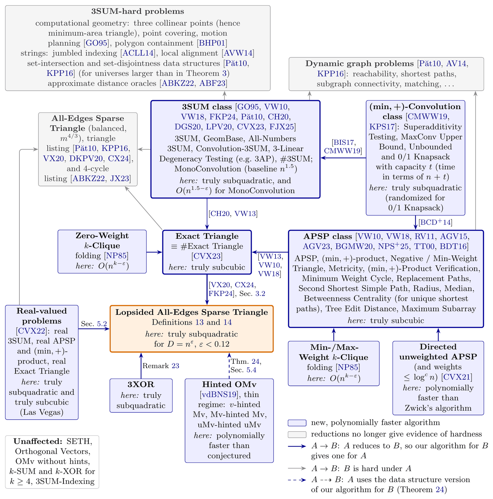
The map is worth reading carefully, because the direction of each arrow decides what happened.
Every problem equivalent to 3SUM or APSP gets a faster algorithm: the whole APSP class (Negative Triangle, Minimum Weight Cycle, Replacement Paths, Second Shortest Simple Path, Radius, Median, Betweenness Centrality for unique shortest paths, Metricity, Tree Edit Distance with integer costs, Maximum Subarray, the Wiener Index) and the whole 3SUM class (GeomBase, All-Numbers 3SUM, Convolution-3SUM, 3-Linear Degeneracy Testing such as finding a 3-term arithmetic progression, and counting 3SUM solutions). Exact Triangle drops to . Zero-, Min- and Max-Weight -Clique fall below through the classical folding into triangles. The -convolution class falls (Superadditivity Testing, Tree Sparsity, Maximum Consecutive Subsums), and with it Knapsack in , randomized for 0/1. Directed unweighted APSP beats Zwick's for the first time in over two decades without help from faster matrix multiplication.
I wondered whether the integer hashing made this an artefact of bounded words. It does not: real numbers fall too. With randomness, Chan, Vassilevska Williams and Xu's reduction from real-valued 3SUM and APSP to sparse triangle counting uses only additions, subtractions and comparisons (Fredman's trick), and the thin-product algorithm counts. The results are Las Vegas algorithms in expected time for real 3SUM and for real APSP and the real product.
Problems that were only 3SUM-hard or APSP-hard get nothing. Three collinear points among points in the plane, the original 3SUM-hard problem, has no new algorithm, because the reduction runs from 3SUM to it. Its bound is now simply unexplained. The same goes for the dynamic graph lower bounds (reachability, shortest paths, subgraph connectivity, matching) and the set-disjointness data-structure bounds for larger universes. Those were the papers whose conclusions depended on the hypotheses, and they now need a different assumption.
Lower bounds in restricted models remain true and matter less. Kerr's bound for straight-line programs and the bound for 3-linear decision trees still hold; the new algorithms escape those models by hashing the weights away and counting triangles with integer matrix products.
SETH and Orthogonal Vectors are untouched, and so are OMv without hints, -SUM and -XOR for , and 3SUM-Indexing. The paper gives reasons rather than hope: 3SUM, APSP and Exact Triangle always had fast nondeterministic and co-nondeterministic algorithms and shallow decision trees (near-linear depth for 3SUM and Exact Triangle, for APSP), while CNF-SAT and OV have neither. It also adds a sharp corollary: if a deterministic fine-grained reduction from CNF-SAT or OV to 3SUM, APSP or Exact Triangle existed, SETH itself would now be false.
Where attention comes in
This last point is the one most readers of this site will care about. The standard argument that exact softmax attention cannot be computed in truly subquadratic time rests on SETH, not 3SUM. Keles, Wijewardena and Hegde (arXiv 2209.04881) prove self-attention is "necessarily quadratic in the input length, unless the Strong Exponential Time Hypothesis (SETH) is false", and Alman and Song (arXiv 2302.13214, the same Alman) show approximate attention with entries of size has no algorithm under SETH. Both bounds survive this paper intact. If you were hoping the quadratic cost of attention had just become negotiable, it has not; the linear-attention designs still pay for subquadratic time with a different, approximate operator.
One attention-adjacent result does fall at the edge. Van den Brand, Song and Zhou proved their data structure for dynamic attention maintenance conditionally optimal under a variant of a hinted OMv conjecture. Section 5.4 shows the new data structure refutes that variant for thin hints, so for that optimality claim "needs a new hypothesis". The algorithm itself is not faster; what changed is the evidence that it could not be beaten.
Who found it
The methodology section is unusually specific, and I think it is the most important paragraph in the paper for anyone outside theory. An Anthropic employee was using an internal research model on open problems in cryptography, one of them about constructions based on the average-case hardness of Zero--Clique. "Claude was tasked with verifying and improving the constructions, but instead developed this algorithm, first for the average case, then for the worst case. The session used 16M output tokens with no human input." Anthropic shared it with the authors in September 2026 under a confidentiality agreement and offered compensation.
The division of labour is stated precisely too. What Claude produced was "essentially the algorithm in
Section 2, although presented differently and with other numerical parameters", plus a different
reduction from Exact Triangle that the authors replaced with the known ones. The data-structure version,
the hinted-OMv consequences and the presentation are the authors'. After the paper was written, a model
certified the main theorems in Lean 4 with Mathlib (Theorem 19, Theorem 22 and the Zero-Weight case of
Corollary 39, with all lemmas they rely on); the formalization is in Anthropic's formal-math
repository under 3sum-apsp. I did not read or build that formalization, so I cannot tell you how
faithfully the Lean statements match the paper's; the Thomson N=7
article is a good reminder that a machine-checked proof is only as good as
its statement.
The irony is hard to miss. The model was asked to make a hardness assumption more useful, and it broke the assumption instead. Cryptography built on fine-grained hardness of Zero--Clique has just lost its worst-case footing, since the paper also refutes the Zero-Weight -Clique hypothesis.
What people are saying
Two days in, I found no written response from a fine-grained complexity researcher outside the author list, and I will not invent one. The paper was discussed on Hacker News within hours. The most useful comments there come from people who read it. User thomasahle summarised the technique accurately: "interpret rectangular matrix algorithms like Schonhage's as a tree, and then very carefully extract only some of the entries." User dgacmu compared it to the early improvements to the matrix multiplication exponent: "it has a very similar feel to Stothers' and then Virginia Williams' earlier improvement on matrix multiply", which reopened a stuck problem without producing anything practical. The sceptical reading came from jltsiren, who called it "an entire house of cards collapsed" for conditional lower bounds and worried that specific formulations of hardness are now "fixed targets for the AI to attack". I think that last worry has it backwards. A hypothesis that falls to a 0.0008 improvement was stated too sharply, and the paper's own conclusion already proposes replacements: restrict the hypotheses to combinatorial algorithms, or move the conjectured hardness to the balanced sparse triangle problem with its bound, which this technique does not touch.
What I take from it
Three things.
The technique is small. Strip away the reductions and the paper's contribution is a counting argument about which leaves of a recursion tree a sparse set of outputs needs, applied to a 1981 identity and a 1982 algorithm (Coppersmith's rectangular multiplication). The authors compare the pruning to FFT pruning and trimmed Möbius inversion. The genuinely new piece is the count in Section 2.4.3. Ideas this small are usually the ones that get improved fast, and the paper says outright that better exponents already exist and were left out for clarity.
Reductions are algorithms. Every arrow in Figure 1 was drawn to prove a lower bound, and every one of them just became a delivery route for an upper bound. The losses those reductions take (a half, a third) suddenly matter, and so does work like Sheffield, Vassilevska Williams and Xi's result that the one-third loss is optimal for black-box reductions.
And the claim at the top of the abstract deserves to be read literally. A model, unprompted, found a polynomial improvement over problems that had resisted the field since the 1970s, and two of the people best placed to judge it (both are co-authors of the current best bounds on ) checked it, simplified it and put their names on it. I have reported on several AI-for-math results on this site. This is the first where the result itself, not the fact that a model found it, is the headline.
How I checked
I read the arXiv HTML and PDF of 2610.06783v1 in full, with Sections 1 to 3 and 4.4 in detail. The five
figures are cropped from the PDF rendered at 300 dpi. In plain Python I wrote out Schönhage's ten
linear forms from Section 2.2 as coefficient tables and compared the expanded left-hand side with
monomial by monomial (they agree on all 33 monomials); implemented the Full recursion of Section
2.3 and checked Lemma 9 against direct matrix products for ; recomputed
and for Figure 6 (1, 18, 81 leaves shared by 1, 5, 15 entries) and the worst ratio
at (0.474 at , below 1/2 for every I tried); evaluated the Lemma
11 sum in log space for the widget; and redid every exponent: , ,
, , , against , , and
. All match the paper. The practicality thresholds are my own
arithmetic from the stated exponents with constants set to 1. I did not read the Lean formalization,
did not verify the reductions I describe as cited, and did not check Sections 5.1 to 5.3 beyond reading
them. The expert-reaction section reflects what I could find on 7 October 2026: the Hacker News threads
and secondary write-ups, none from named researchers in the area.