Functional gradient descent: refine the gradient until the step is safe

2026-09-27 · 21 min · explainer · theory · math · training · pde · 3d

"Functional GD algorithms generally outperform neural nets, but are hard to accurately implement. We fix this!" That is Daniel Csillag announcing Functional Gradient Descent with Adaptive Representations (arXiv 2606.16926), written with Rodrigo Schuller, Pedro Dall'Antonia, Leonidas Guibas, Luiz Velho and Tiago Novello at FGV EMAp, IMPA and Stanford.

The fix is narrower than the post, and more interesting. Gradient descent in function space has clean theory, but the gradient it needs is a function, and a program can only hold an approximation of it. Every earlier implementation fixed that approximation up front, and a fixed approximation puts a floor under the loss. Instead, before each step it bounds the error of what it stored, and it refines the representation until that bound is a small fraction of the stored gradient. With that one rule, the standard convergence proofs survive.

I read the paper, rebuilt its toy setting in one dimension so you can watch the algorithm run, and checked each "outperforms" against the paper's own figures.

Two places to take a gradient step

You want a function $f$ that minimises a loss $L(f)$ : a regression fit, a PDE residual, a photometric error over a radiance field. The usual move is to pick a parameterised family $f_\theta$ , a neural network, and run gradient descent on the weights:

\theta_{t+1} = \theta_t - \eta \, \nabla_\theta L(f_{\theta_t}).

The alternative is to step the function directly:

f_{t+1} = f_t - \eta \, \nabla L(f_t),

where $\nabla L(f_t)$ is a function of the same kind as $f_t$ . That is functional gradient descent, FGD.

The first reason to care is convexity. If the pointwise loss $\ell(\hat y, y)$ is convex in $\hat y$ , then $L(f) = \int \ell(f(x), y(x))\,dx$ is convex in $f$ , because evaluating $f$ at a point is linear in $f$ . Parameterising breaks that. The smallest example I know: fit $y(x) = x$ on $[0,1]$ with $f(x) = c\,x$ . In function space the loss is $(c-1)^2/6$ , a parabola. Now write $c = a\,w$ , a two-layer linear "network". The loss $(aw-1)^2/6$ is zero at $(a,w) = (1,1)$ and at $(-1,-1)$ , and it is $1/6$ at their midpoint $(0,0)$ . A convex function cannot do that. Same function class, same loss, and the parameterisation alone made it nonconvex (reasoned).

The second reason is that parameter-space descent is already a function-space method, seen through a lens. By the chain rule, one weight step moves the function, to first order, by

f_{\theta_{t+1}}(x) - f_{\theta_t}(x) \approx -\eta \int \Theta_t(x, x') \, [\nabla L(f_{\theta_t})](x') \, dx', \qquad \Theta_t(x, x') = \partial_\theta f_{\theta_t}(x)^\top \partial_\theta f_{\theta_t}(x').

$\Theta_t$ is the neural tangent kernel (Jacot et al., 2018). Gradient descent on a network is functional gradient descent preconditioned by a kernel the network chooses, and that kernel changes every time the weights move. FGD drops the lens and steps along the gradient itself.

What a functional gradient is

For a loss on a space of functions $\mathcal H$ , the directional derivative is

\mathrm{D}L(f; h) = \lim_{\delta \searrow 0} \frac{L(f + \delta h) - L(f)}{\delta}.

When $\mathcal H$ is a Hilbert space and $\mathrm{D}L(f;\cdot)$ is a continuous linear map, the Riesz representation theorem gives a unique element $\nabla L(f) \in \mathcal H$ with $\mathrm{D}L(f; h) = \langle \nabla L(f), h \rangle_{\mathcal H}$ for every $h$ . That element is the functional gradient: the Riesz representer of the derivative. In $\mathbb R^d$ with the dot product it is the ordinary gradient.

The inner product decides what the gradient looks like, and the paper's two main examples show it.

$L^2$ . For the fitting loss $L(f) = \tfrac12 \|f - f^\star\|_{L^2}^2$ , the derivative is $\int (f - f^\star)\,h$ , so $\nabla L(f) = f - f^\star$ : the residual. The paper also shows (its Proposition A.1) that $L - L^\star = \tfrac12 \|\nabla L\|^2$ here, the Polyak-Łojasiewicz condition with constant 1.

An RKHS. The empirical loss $\frac1n \sum_i \ell(f(X_i), Y_i)$ does not even make sense in $L^2$ , whose elements have no values at single points. In a reproducing kernel Hilbert space $\mathcal H_K$ , evaluation is an inner product, $f(x) = \langle f, K(x,\cdot) \rangle$ , and the gradient comes out as a sum of kernel bumps centred on the data (Proposition 4.1):

[\nabla L(f)](x) = \frac1n \sum_{i=1}^n \ell'(f(X_i), Y_i)\, K(X_i, x).

Same loss, different geometry, different gradient. Muon is the parameter-space cousin of this idea: it reshapes the update instead of taking the raw gradient, which amounts to measuring the step in a different norm.

Why the gradient cannot be stored

$\nabla L(f_t)$ is a function, so in general it is infinite-dimensional. The iterate $f_t = f_0 - \eta \sum_{s<t} g_s$ also carries every past step. The RKHS case is the lucky exception: the gradient above is exactly $n$ kernel bumps, so exact FGD is kernel regression by gradient descent. The paper notes that such approaches "rely on specific finite-sample structures" and scale poorly with sample size. A Sobolev-space PDE loss or a radiance field has no such finite form.

So implementations approximate. The families I know:

Boosting. Mason et al. (1999) showed that AdaBoost-style boosting is gradient descent in function space, and Friedman's gradient boosting machine (2001) is built on that reading. Each round fits a small tree to the negative gradient at the data and steps along the tree. A depth-limited tree is a fixed-capacity approximation of the gradient. The paper does not cite this line, but its fixed-depth tree baselines are the same move. Gradient-boosted trees are still what TabFM has to beat on tables.
Kernel methods. Exact in an RKHS, as above, at a cost that grows with $n$ .
Fixed grids or bases. Project the gradient onto a fixed grid, step, repeat. This is the paper's "Approx. FGD" baseline.
The network itself. The NTK view above: a parameterisation is a representation, fixed a priori, with a kernel that moves.

The approximate-FGD work the paper does cite (Fonseca and Saporito 2022; Peixoto et al. 2024 and 2025; Petrulionyte et al. 2024; Kim et al. 2025) has, it argues, irreducible approximation error that the analysis usually leaves out.

For the $L^2$ fit you can see the floor in one line (reasoned). On a fixed grid that reads $f^\star$ at cell midpoints, the stored gradient is $g_t = f_t - P f^\star$ , where $P f^\star$ is $f^\star$ read that way. The iteration converges to $P f^\star$ and the loss stops at $\tfrac12 \|f^\star - P f^\star\|^2$ , however long you run it. A finer grid lowers the floor but does not remove it.

The algorithm: refine until the error is a fraction of the step

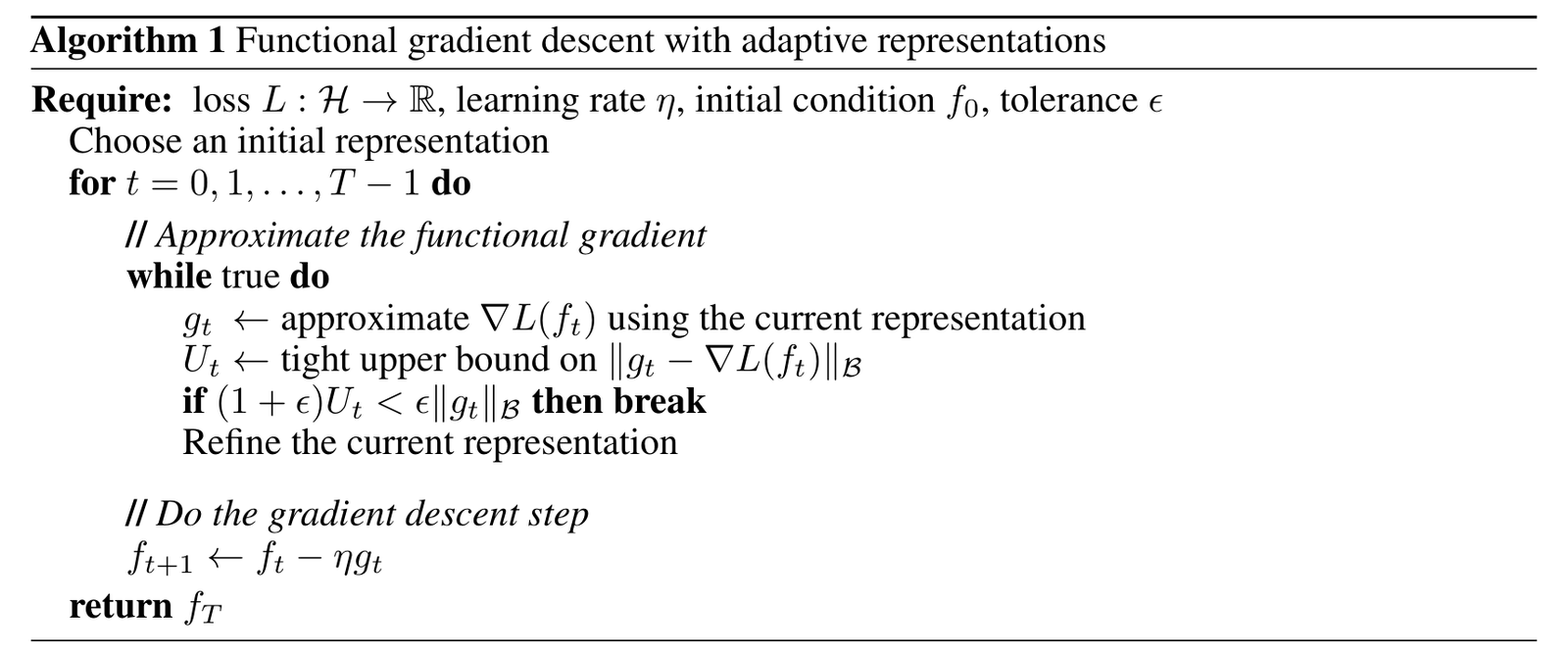
Algorithm 1, functional gradient descent with adaptive representations. Require: loss L from H to R, learning rate eta, initial condition f0, tolerance epsilon. Choose an initial representation. For t from 0 to T minus 1: while true, set g_t to an approximation of grad L of f_t in the current representation, set U_t to a tight upper bound on the B-norm of g_t minus grad L of f_t, break if one plus epsilon times U_t is less than epsilon times the B-norm of g_t, otherwise refine the current representation. Then set f_t+1 to f_t minus eta g_t. Return f_T. — The whole method. The inner loop refines until the certified error bound U is small against the size of the stored gradient; only then does the step happen (paper, Algorithm 1).

Three pieces make this work.

A test you can compute. The relative error $\mathrm{RelErr}(g, \nabla L(f)) = \|g - \nabla L(f)\|_{\mathcal B} / \|g\|_{\mathcal B}$ divides by the norm of the stored gradient, which you can compute exactly, not the true one, which you cannot. The numerator is replaced by an upper bound $U$ that the representation can certify: a Lipschitz constant per tree leaf, a tail bound on a Fourier transform. The step runs only when $(1+\epsilon)\,U_t < \epsilon \|g_t\|_{\mathcal B}$ .

A loop that ends. Lemma 3.9 says that if the refinements drive $U$ to zero, some refinement passes the test. The proof divides by the norm of the true gradient, so it assumes that gradient is not zero; at an exact stationary point there is nothing to step toward anyway.

Two spaces. The gradient lives in a Hilbert space $\mathcal H$ , because it needs an inner product. The approximation lives in a larger Banach space $\mathcal B$ , because that is where the useful representations are. Piecewise-constant trees are in $L^\infty$ but not in an RBF kernel's RKHS. Two constants tie the spaces together: $\alpha$ says the extended gradient is still a descent direction measured in $\mathcal B$ , and $\beta$ bounds the derivative's dual norm by the gradient's norm. Both equal 1 when $\mathcal B = \mathcal H$ .

What "the representation" is differs by experiment. The paper describes each only briefly:

Task	Function space	What stores $g_t$	How it refines	How $U$ is bounded
2-D toy fit	$L^2([0,1]^2)$	a uniform grid, judging by Figure 1	a finer grid	not described
RKHS regression	RBF kernel $\exp(-100 \lVert x-y \rVert^2)$ , approximated in $L^\infty$	trees with splits at midpoints	deeper trees	per-leaf Lipschitz bound, from the kernel's Lipschitz constant
Wave equation	Sobolev $H^2(\mathbb R^3)$	piecewise-constant Fourier transform on a uniform frequency grid, inverted as a sum of sincs	a finer frequency grid	Lipschitz bound inside the grid plus a bound on the Sobolev symbol outside it
Radiance field	density in $L^2$ , colour with an RKHS over view directions	uniform 3-D grids, spherical harmonics per voxel for colour	a finer grid	not described

(reported, paper Sections 4.1 to 4.3 and Appendix B).

The guarantee, stated precisely

The assumptions, all on the larger space $\mathcal B$ : $L$ and $\nabla L$ extend from $\mathcal H$ to $\mathcal B$ (3.1); $L$ is $K$ -smooth, $L(f) \le L(f') + \mathrm{D}L(f'; f - f') + \tfrac K2 \|f - f'\|_{\mathcal B}^2$ (3.2); $\mathcal H$ descends in $\mathcal B$ , $\mathrm{D}L(f; \nabla L(f)) \ge \alpha \|\nabla L(f)\|_{\mathcal B}^2$ (3.3); and gradient compatibility, $\|\mathrm{D}L(f;\cdot)\|_{\mathcal B^*} \le \beta \|\nabla L(f)\|_{\mathcal B}$ (3.4). For the global result add a Polyak-Łojasiewicz condition, $L(f) - L^\star \le \tfrac{1}{2\mu} \|\mathrm{D}L(f;\cdot)\|_{\mathcal B^*}^2$ with $L^\star = \inf_{\mathcal H} L$ (3.7).

Theorem 3.10 then says, for Algorithm 1 with tolerance $\epsilon \in (0,1)$ :

Relative error. Every step has $\mathrm{RelErr}(g_t, \nabla L(f_t)) \le e := \epsilon/(1+\epsilon)$ , which is below $1/2$ .
Stationarity. If $L \ge L^\star$ , $e < \min\{1/2,\ \alpha/(\alpha+\beta)\}$ and $\eta < 2(\alpha - (\alpha+\beta)e) / (K(2e+1))$ , then

\min_{t < T} \|\nabla L(f_t)\|_{\mathcal B}^2 \le \frac{L(f_0) - L^\star}{T \eta r}, \qquad r = \alpha - \frac{K\eta}{2} - \Big(\beta + \frac32 K\eta\Big) \frac{e}{1-e} > 0 .

Global minimum. Under the Polyak-Łojasiewicz condition as well,

L(f_T) - L^\star \le \big(1 - 2\eta\beta^{-2}\mu r\big)^T \big(L(f_0) - L^\star\big).

The engine is Lemma 3.5, a one-step descent lemma with the relative error inside the bracket. It is tight in the sense the paper states: with $\mathcal B = \mathcal H$ , an exact gradient and $\eta = 1/K$ , it collapses to the textbook $L(f_{t+1}) \le L(f_t) - \frac{\eta}{2}\|\nabla L(f_t)\|^2$ .

A worked instance, which is also the widget below (reasoned). For the $L^2$ fit, $\alpha = \beta = K = \mu = 1$ . Take $\epsilon = 0.5$ , so $e = 1/3$ , which is under $1/2$ . The step-size condition becomes $\eta < 2(1 - 2/3)/(2/3 + 1) = 0.4$ . At $\eta = 0.25$ , $r = 1 - 0.125 - 1.375 \times 0.5 = 0.1875$ , and the guaranteed contraction is $1 - 2 \times 0.25 \times 0.1875 = 0.90625$ per step.

What the theorem does not say is as important:

It counts steps, not work. Lemma 3.9 promises the inner loop ends, not when. As $\|\nabla L\|$ shrinks, $U$ has to shrink with it, so the representation keeps growing for as long as the loss keeps falling.
Its constants can be ruinous. For the RKHS experiment, Proposition A.2 gives $\alpha = \lambda_{\min}(K)/(n\kappa^2)$ and $\beta = n/\lambda_{\min}(K)$ . For an RBF kernel, $\kappa = 1$ and $\lambda_{\min} \le 1$ , so $\alpha/(\alpha+\beta) \le 1/(1+n^2)$ (reasoned). With a thousand training points, the relative error the theorem needs is about one in a million, and the step size must be below $2\alpha/K$ , which is at most $2/(nK)$ ( $K$ here is the smoothness constant, not the kernel). The paper tunes learning rates "to obtain the best possible performance" and does not report $\epsilon$ or $n$ for this run, so I cannot tell whether the experiment ran inside the theorem.
It covers two of the four experiments. The paper proves the Polyak-Łojasiewicz condition for the $L^2$ toy and for RKHS regression with a strongly convex $\ell$ . It does not claim it for the wave equation. The radiance-field loss is, in the paper's words, "highly nonconvex", so the global result does not apply there, and $K$ -smoothness is not checked for it either.

Running it in one dimension

The paper's toy problem fits a spiral on the unit square. The widget runs the same kind of fit in one dimension, entirely in your browser. The target $f^\star$ on $[0,1]$ has three scales: a gentle sine, a sharp step at $x = 0.3$ , and a wave packet near $x = 0.72$ . The loss is $\tfrac12 \|f - f^\star\|_{L^2}^2$ , so the functional gradient is the residual. Four methods start from $f_0 = 0$ :

Adaptive FGD is Algorithm 1. $g_t$ is piecewise constant on dyadic cells and reads $f^\star$ at cell midpoints. $U$ comes from a per-cell Lipschitz bound on $f^\star$ , and the refinement splits the cell with the largest share of $U^2$ . It uses $\epsilon = 0.5$ and $\eta = 0.25$ , the worked instance above, and no cell may be narrower than 1/1,024.
Fixed grids of 16 and 128 cells take the same step and never refine.
A ReLU network with 16 hidden units is trained on the same loss with full-batch Adam. Its learning rate, 0.02, gave the best final loss of the five I tried (0.01, 0.02, 0.05, 0.1 and 0.2).

fitting f* on [0, 1] · gradient descent in function spaceruns in your browser

step t6

loss L(f_t)

1.42×10⁻³

Theorem 3.10 bound

2.38×10⁻²

cells in g_t

140

cells split this step

certified U / ‖g_t‖

0.332

The loss is ½‖f − f*‖², so the functional gradient is the residual f_t − f* itself. Each grid method stores a piecewise-constant g_t, read at cell midpoints, and steps f ← f − 0.25·g_t. The adaptive run splits its worst cell until a certified bound on the storage error is under a third of ‖g_t‖ (the paper’s test with ε = 0.5); the fixed grids never split, so that ratio climbs past the threshold and their loss stalls. The network is trained on the same loss with Adam at 0.02. The dashed line is the rate Theorem 3.10 guarantees, 0.90625 per step, far looser than what the run achieves. It stops applying once cells reach their minimum width of 1/1,024 and the test can no longer pass; from there the adaptive run is a fixed grid too.

The top panel is $f_t$ against the target, with ticks marking cell edges or, for the network, its kinks. The middle panel is the true gradient $f_t - f^\star$ as a thin line and, for the grids, the stored $g_t$ as a thick one; the gap between them is what $U$ has to cover. The bottom panel is the loss of all four on a log scale. What it shows, from running the same code under Node 22 (measured):

The test forces refinement from the start. At step 0 the adaptive run splits 31 times, to 32 cells, before its first step. By step 11 it holds 598 cells, and the loss has fallen from $4.30 \times 10^{-2}$ to $8.42 \times 10^{-5}$ .
The refinement goes where $f^\star$ is steep. At step 8, cells are 1/1,024 wide around the step at $x = 0.3$ , narrower than average in the wave packet, and 1/128 wide on the gentle stretches.
Fixed grids fail the test and then stall. The 16-cell grid's certified ratio $U/\|g\|$ is 1.44 at step 0, above the threshold of one third before it moves, and its loss stops at $3.89 \times 10^{-3}$ . The 128-cell grid passes the test through step 3 and fails it from step 4. It keeps pace with the adaptive run through step 6 ( $1.43$ against $1.42 \times 10^{-3}$ ), then stops at $8.49 \times 10^{-5}$ .
The guarantee is loose. At step 11, Theorem 3.10 allows $1.46 \times 10^{-2}$ ; the run is at $8.42 \times 10^{-5}$ , about 170 times lower (reasoned from the two).
The guarantee ends where the memory does. At step 12 the loop splits 426 more times, every cell reaches the 1/1,024 minimum, and the ratio still reads 0.347. From there the run is a uniform 1,024-cell grid, and it flattens at $1.00 \times 10^{-6}$ . The relative test is global: once the residual is small everywhere, even the flat stretches need refining.
The network is slowest per step. After 40 Adam steps it is at $5.03 \times 10^{-3}$ , behind even the 16-cell grid. A network step is cheaper than a refinement loop, so this is a per-step comparison, the same axis the paper plots.

The last two points are the method's real cost. The certificate is honest, and the price of honesty is a representation that grows until you stop it.

What "outperforms neural nets" means, experiment by experiment

The experiments ran on one desktop with an Intel Core i9-14900KF and an RTX 4090 (reported).

Left: three rows of four heatmaps of a spiral at optimisation steps 10, 25, 50 and 100. The neural-network row reaches loss 9e-4 in 1.9 s, the fixed-representation FGD row loss 5e-3 in 262 ms, and the adaptive row, which starts blocky and sharpens, loss 1e-5 in 417 ms. Right: training loss on a log scale against optimisation steps. Fixed-grid FGD curves for 16 squared up to 512 squared grids fall fast and flatten at successively lower floors; the neural-network curve, marked sped up 4x, falls slowly; the adaptive curve falls to a dashed line labelled global minimum. — The toy problem: fitting a spiral in L² on the unit square. Fixed grids converge quickly to their own floors; the adaptive run starts coarse and keeps going. The network curve is marked as sped up 4x on the step axis (paper, Figure 1).

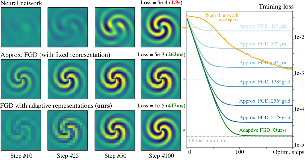
The 2-D toy fit (reported). The printed losses are $9 \times 10^{-4}$ for the network in 1.9 s, $5 \times 10^{-3}$ for the pictured fixed grid (its arrow points at the 32² curve) in 262 ms, and $1 \times 10^{-5}$ for adaptive FGD in 417 ms. That is about 90 times lower loss, 4.6 times faster (reasoned). The network's curve has not flattened when the plot ends.

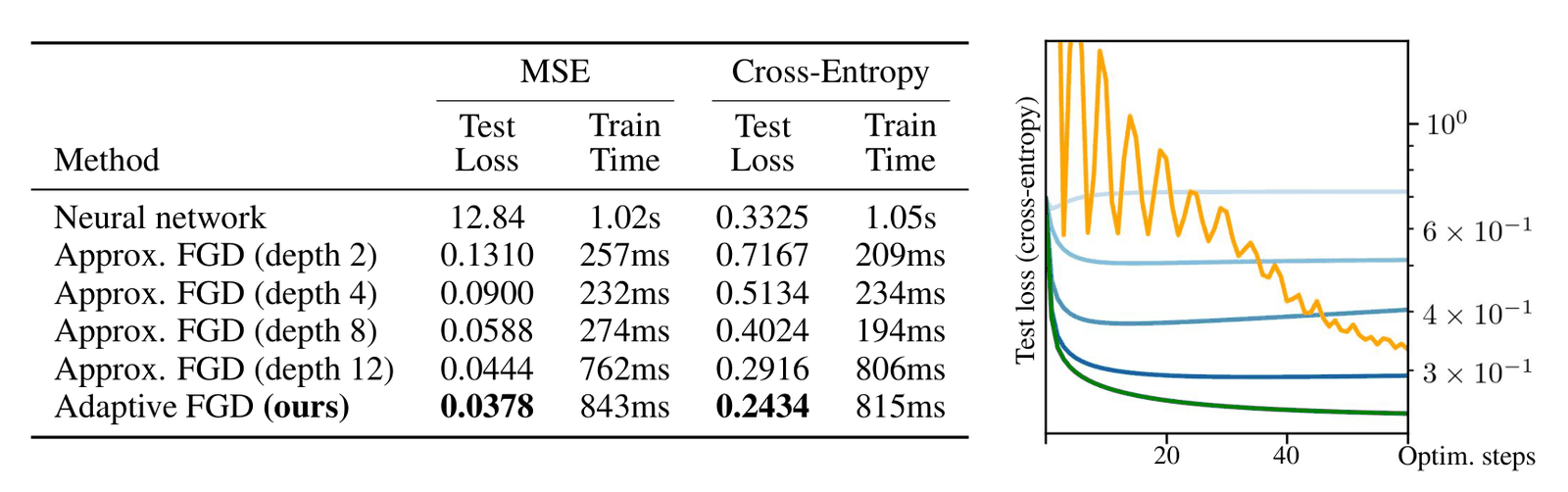
A table and a plot. The table lists test loss and train time for MSE and cross-entropy: neural network 12.84 and 1.02s, 0.3325 and 1.05s; approximate FGD at tree depth 2: 0.1310 and 257ms, 0.7167 and 209ms; depth 4: 0.0900 and 232ms, 0.5134 and 234ms; depth 8: 0.0588 and 274ms, 0.4024 and 194ms; depth 12: 0.0444 and 762ms, 0.2916 and 806ms; adaptive FGD: 0.0378 and 843ms, 0.2434 and 815ms. The plot shows cross-entropy test loss against optimisation steps: the network oscillates widely before settling near 0.33; fixed-depth curves flatten at different levels; the adaptive curve is lowest. — Regression in an RKHS on a non-coding RNA classification set, with trees as the adaptive representation and a two-hidden-layer MLP as the network (paper, Figure 2).

RKHS regression (reported). The data is the LIBSVM set for detecting non-coding RNA sequences; the network is an MLP with two hidden layers of 256. With cross-entropy, adaptive FGD reaches a test loss of 0.2434 against 0.3325 for the network, 27% lower (reasoned), in 815 ms against 1.05 s. Three things temper that. The network beats the fixed trees of depth 2, 4 and 8 (0.7167, 0.5134 and 0.4024), so "functional GD generally outperforms neural nets" does not hold for fixed-representation FGD even here. Adaptive FGD is the slowest FGD row, 843 ms on MSE against 232 to 762 ms for the fixed trees. And the network's MSE test loss is 12.84. With the paper's $\tfrac12(\hat y - y)^2$ , that is a root-mean-square error of about 5 on a binary target (reasoned): that baseline did not fit, and the paper does not discuss it.

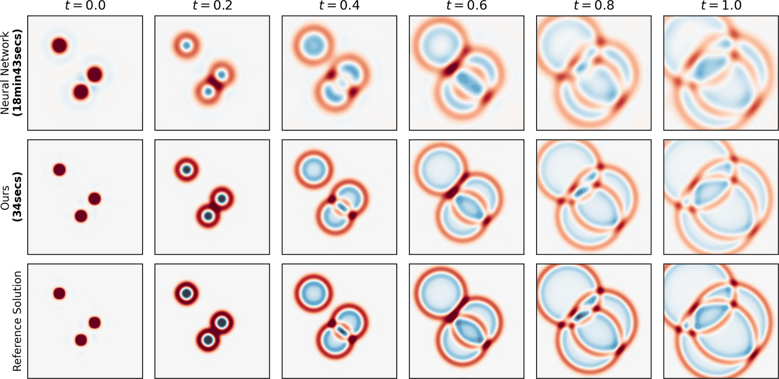
Three rows of six snapshots of a 2-D wave field at t = 0.0, 0.2, 0.4, 0.6, 0.8 and 1.0, starting from three blobs that expand into interfering rings. Top row: neural network, 18 min 43 secs, with blurred rings and faint artefacts. Middle row: ours, 34 secs. Bottom row: reference solution. The middle row closely matches the reference. — The wave equation from three initial blobs. The network baseline needed a Fourier-feature embedding to fit at all. No error numbers are reported for this experiment (paper, Figure 3).

The wave equation (reported). The loss is the squared PDE residual plus the two initial conditions, over $H^2(\mathbb R^3)$ , and the gradient has a closed-form Fourier transform (Proposition 4.2). Figure 3's labels read 18 min 43 s for the network and 34 s for adaptive FGD, about 33 times faster (reasoned). The text calls it "nearly two orders of magnitude"; 33 times is about one and a half. There is no error number, only pictures against a finite-difference reference. The text also says fixed-representation FGD "quickly plateaus" here, but no figure or table in the paper shows it. For the physics-informed side of this, Lanyon comes at PDE solvers from the opposite end: proving the numerics correct rather than learning them.

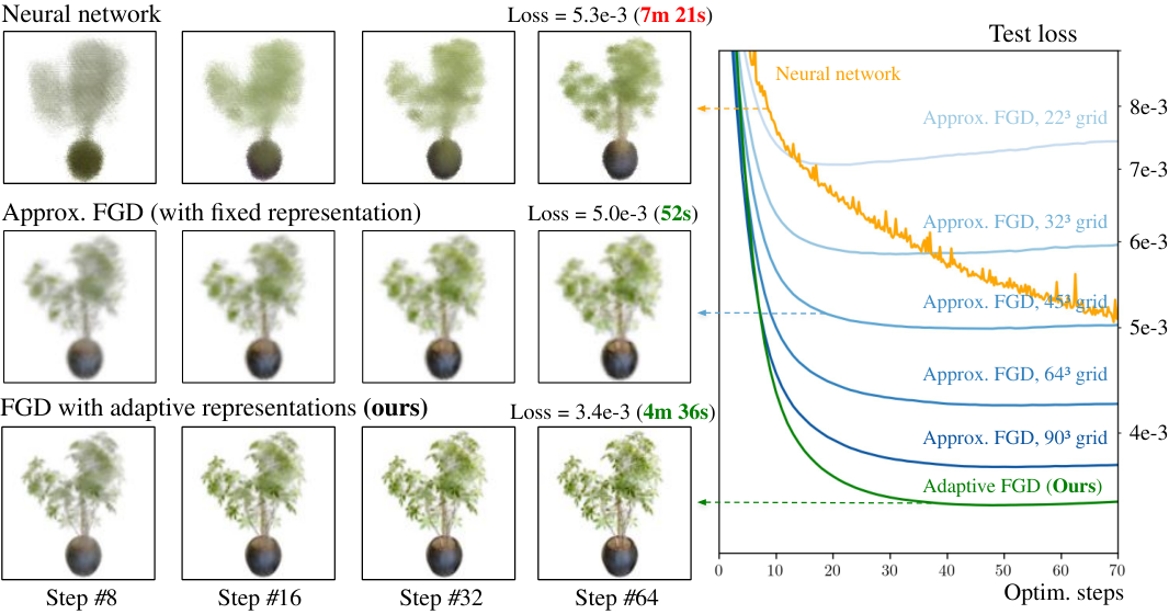
Left: three rows of four novel-view renders of the Ficus plant at steps 8, 16, 32 and 64. Neural network, loss 5.3e-3 in 7 m 21 s, stays hazy. Fixed-representation FGD, loss 5.0e-3 in 52 s, is blurry. Adaptive FGD, loss 3.4e-3 in 4 m 36 s, is the sharpest. Right: test loss against optimisation steps up to 70. Fixed grids from 22 cubed to 90 cubed flatten at decreasing levels; the neural network curve is noisy and still falling at step 70; the adaptive curve is lowest. — Inverse rendering of the Ficus scene: density and view-dependent colour stepped directly in function space, against a network trained with Adam and against fixed grids (paper, Figure 4).

Radiance field (reported). The Ficus scene from NeRF-Synthetic, trained on 24 views at 160×160 and tested on 25 others. The printed test losses are $5.3 \times 10^{-3}$ for the network in 7 m 21 s, $5.0 \times 10^{-3}$ for the pictured fixed grid (its arrow points at the 45³ curve) in 52 s, and $3.4 \times 10^{-3}$ for adaptive FGD in 4 m 36 s. So adaptive FGD is 36% lower than the network and 1.6 times faster, and 5.3 times slower than the fixed grid it beats (reasoned). One network step is 96 mini-batches of 80×80 rays, which is exactly the 614,400 training rays, so over the plotted 70 steps the network saw 70 epochs of Adam at $10^{-4}$ , and its curve is still falling at the right edge. If the plotted loss is Equation 10 with colours in $[0,1]$ , those losses are roughly 26.4 dB and 24.5 dB PSNR (reasoned, on that assumption); the paper reports no PSNR. More radiance-field work is in the 3D reconstruction roundup.

Task	Metric	Network	Fixed-representation FGD	Adaptive FGD	Time, network vs adaptive
2-D toy fit	training loss	$9 \times 10^{-4}$	$5 \times 10^{-3}$ (pictured 32² row)	$1 \times 10^{-5}$	1.9 s vs 417 ms
RKHS, MSE	test loss	12.84	0.0444 (best, depth 12)	0.0378	1.02 s vs 843 ms
RKHS, cross-entropy	test loss	0.3325	0.2916 (best, depth 12)	0.2434	1.05 s vs 815 ms
Wave equation	none reported	pictures	not shown	pictures	18 min 43 s vs 34 s
Radiance field	test loss	$5.3 \times 10^{-3}$	$5.0 \times 10^{-3}$ (pictured 45³ row)	$3.4 \times 10^{-3}$	7 m 21 s vs 4 m 36 s

(reported; the ratios in the prose are reasoned). The paper gives one number per method, with no seeds or spread. So "outperforms neural nets" means this: on four problems whose gradient has a closed form that a grid or a tree can hold, adaptive FGD beat a tuned network on loss (on pictures, for the wave equation) and on wall-clock. In two of them the network's curve was still falling when the comparison stopped, and in one it did not fit at all.

What I could not check

The code. The paper points to dccsillag/experiments-adaptive-fgd on GitHub. On 27 September 2026, git clone asks for credentials and the repository is not among the author's 29 public ones (measured), so none of the numbers above could be re-run.
The venue. The first author announced the NeurIPS acceptance on X on 26 September 2026 (reported). The arXiv v1 PDF, submitted 15 June, predates it: it is still marked "Preprint", and the abstract page lists no journal reference yet.
The unreported settings. $\epsilon$ for every experiment, $n$ and the test split for the RKHS run, and the error bounds for the toy and radiance-field representations are not in the paper.

Where it breaks, and what it costs

The contribution is a rule, not a representation: store the gradient however you like, as long as you can certify an upper bound on the error and drive it to zero. That turns an approximation that used to cap the loss into one that only costs memory. It also moves the hard part. For each new loss you need a representation whose error you can bound, which the paper supplies for kernels, Fourier grids and voxel grids but not in general. And you have to accept that the representation grows for as long as the loss falls. My 1-D run needed its finest grid everywhere by step 12.

What I would want next is a version with a budget: the paper's theorem with the refinement cost inside it, so that "converges" comes with a bill.