2026-10-23 · 20 min · flow-matching · diffusion · distillation · image-generation · math
A 1:50 narrated explainer, drawn in code. Every number and picture in it is this article's own; the sources are below.
› transcript
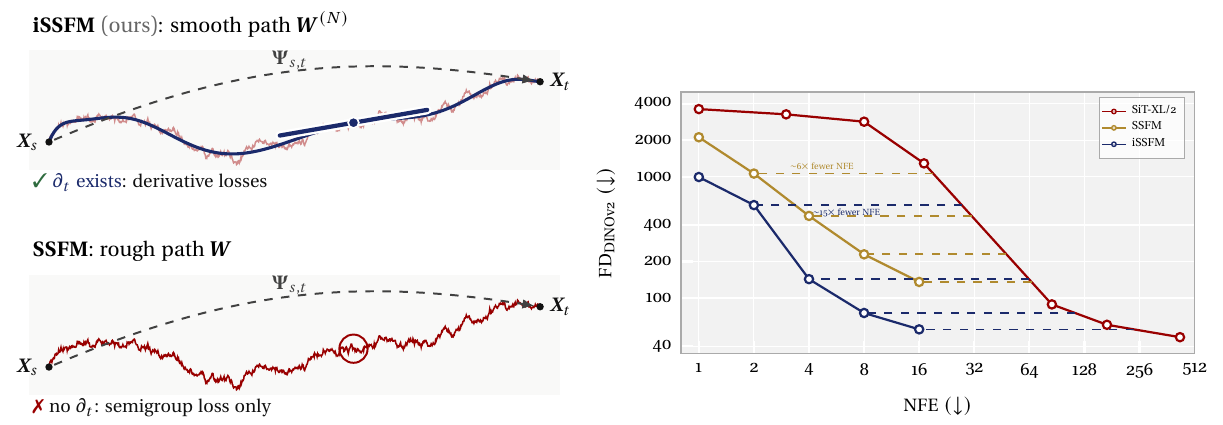
Hi, I'm Transom! A stochastic flow map jumps a noisy process forward in a few big steps. Here's how it got the best training loss. Brownian motion has no slope anywhere. So replace it with a smooth polynomial that converges to it, and train against that. The first paper used a semigroup loss. One big step must equal two half steps. No derivative needed. The new paper trains the flow map of a random ordinary differential equation. Its slope exists, and every coefficient enters the loss. Here is the equation the map now learns. The first term is the usual drift. The second is the slope of the polynomial path. As the degree grows, the solution converges to the true stochastic one. Summarise the noise on the step as three Legendre coefficients. They enter a pretrained flow model through a residual that starts at zero, so the model begins as its teacher. The noise term is computed exactly, from the same path, not learned by a head. Drift plus exact noise gives the next state, in one network call. Top, the smooth path, where a derivative loss exists. Bottom, the rough path, where only the semigroup loss works. On ImageNet, the improved map sits below the original at every step count. At four steps, the new parameterisation and the new loss each roughly halve the error, against the authors' own port of the original. Turn the noise into an input the derivative can see, and a stochastic map trains like a deterministic one. A polynomial path, a derivative loss, and exact noise. That's the improved strong flow map. Every source is in the full article. I'm Transom. Bye!
Why read this
Notabletop 60%The Wong-Zakai loss derived and shown on a live path, every ImageNet ratio rechecked, a swapped legend found in the source, and the toy losses run on CPU.
- Original analysis
- A lasting reference
- A new technique
Image & video generationNeeds datacenter GPUsMITResearch paper
How this was scored
- Is it new?
- 2 of 3: A real new idea, method or capability
- Can I trust it?
- 2 of 3: Measures key facts from files, code or configs
- Can I run it?
- 1 of 3: API-only, gated or restrictive licence
- Will I understand it?
- 2 of 3: Mechanism from first principles with figures
- Can I act on it?
- 2 of 3: A concrete recipe, numbers or comparison
- Will it last?
- 2 of 3: A reference for a year or more
- Does it affect many?
- 1 of 3: A specialist community
- Only here?
- 2 of 3: A teardown or measurement few others did
Score 64 of 100, ranked 254 of 607 rated articles. Each question is answered 0–3 by hand, and a 3 is rare. How articles are scored
A deterministic flow map learns to jump an ODE from time to time in one network call. The strongest recipes for training one, MeanFlow and its improved version, differentiate the map with respect to its start time. A strong stochastic flow map (SSFM) does the same for an SDE: it jumps from to along one specific realisation of the Brownian motion. That is where the derivative breaks. The map depends on the Brownian path between and , and a Brownian path has no derivative anywhere.
The original Strong Stochastic Flow Maps paper (McCallum, Blasingame, Herschell, Rindtorff, Tong and Foster) sidestepped this by training with a semigroup loss: one big step must equal two half steps. The follow-up, Improved Training of Strong Stochastic Flow Maps by Zander W. Blasingame, Antonio Franca, Raúl Miñán, Christian Koke, Niklas Rindtorff and Alexander Tong (AITHYRA, TU Wien, TU München, MCML), gets the derivative losses back. Blasingame's thread calls the first paper a NeurIPS 2026 Oral; its arXiv listing says only "Preprint", so I have not confirmed the venue. Code is at zblasingame/improved-strong-stochastic-flow-maps (MIT) and the five ImageNet checkpoints at zblasingame/improved-strong-stochastic-flow-maps on Hugging Face.
- license
- MIT
- branch
- HEAD
- tests
- none found
- source
- 874.4 kB
- commit date
- 2026-10-22
by size of tracked source at this commit, file counts in brackets; docs, data and vendored trees excluded
local clone, 2026-10-23 at cb7b92d — branch, commit, commitDate, fileCount, hasTests, languages, license, licenseFile
- task
- unconditional-image-generation
- library
- pytorch
- license
- mit
- safetensors
- 5 shards
- largest file
- 165.0 MB
- files
- 12
- downloads
- 0
- likes
- 2
repo last modified 2026-10-22
The same group's Langevin Flow Maps used the SSFM machinery for molecular dynamics. This piece is about the training method underneath. I read the paper and its LaTeX source, read the code, pulled the checkpoint headers, and ran the authors' toy-1D losses on a CPU. Numbers are labelled measured (I computed it from a file or a run), reported (the authors' figure) or reasoned (my arithmetic on the other two).
The short version: a classical theorem, used well. Replace the rough path with a smooth polynomial that converges to it, train against the random ODE that polynomial drives, and the derivative exists. On ImageNet-256 that gives about three times lower FD-DINOv2 than SSFM at 4 and 8 steps, against the authors' own port of SSFM. The "fifteen times fewer steps" is read off an interpolated curve of the weakest available baseline.
Flow maps, deterministic first
Flow matching learns a velocity field whose ODE carries noise () to data (). The interpolant is ; on ImageNet the schedule is linear, , . Sampling integrates the ODE, which costs one network call per solver step.
A flow map skips the solver. It learns the two-time map
where is the mean velocity over . On the diagonal, , the ordinary flow-matching field. Three conditions characterise the true map, and each becomes a loss (reported, Appendix A.2). Write and for the instantaneous field:
- Eulerian: . Moving the start point along the flow does not change where you land.
- Lagrangian: . The endpoint moves with the flow.
- Semigroup: . One big step equals two smaller ones. This is the shortcut model loss, and it needs no derivative.
Improved MeanFlow (iMF) rewrites the Eulerian residual in terms of . With the material derivative , it becomes
with a stop-gradient: regress onto the instantaneous field, corrected by a forward-mode JVP of the network itself. The paper calls this Eulerian family the most performant at scale.
The stochastic version, and why the derivative was missing
Every flow-matching ODE has an SDE with the same marginals (the paper's Equation 1):
For the linear schedule, , which blows up as (reported, Appendix B.4.1).
A weak stochastic flow map learns to sample given : right in distribution, with fresh noise every call. A strong one learns the pathwise solution: given and the Brownian path , return the that this path produces. Step 4 times or 16 times along the same path and you should land on the same sample.
SSFM writes the map as an Euler-Maruyama-shaped step with learned averages:
where is a finite summary of the path on and was a learned diffusion head.
The summary is the shifted Legendre expansion (Foster, Lyons and Oberhauser). Its coefficients are Itô integrals of the Legendre polynomials against the path:
is the increment . The higher ones describe how the path bends away from the straight chord. They are independent, and two intervals' coefficients combine into the parent's by a closed-form Chen relation, which is all the semigroup loss needs (the Langevin Flow Maps piece covers both properties).
Now try the Eulerian loss. It needs : slide the start point and see how the output changes. But takes the path on as input, so sliding changes the path the map sees, and the rate of that change is , which does not exist. The paper also cites Itô maps for any-step SDEs (Pan et al.), whose Proposition 2 shows that a naively applied Eulerian loss places no pathwise constraint on the map: it can be satisfied while ignoring the path.
The fix: train against a random ODE
Step one: give the path a derivative. The degree- Legendre polynomial built from the first coefficients is a smooth curve. For a sub-interval of it is (the paper's Equation 3)
and its time derivative is an ordinary polynomial, in closed form (Lemma B.1):
Step two: replace the SDE with the ODE this derivative drives. Write for the SDE's drift. The Wong-Zakai random ODE on is
Wong and Zakai showed in 1965 that ODEs driven by smooth approximations of Brownian motion converge to the Stratonovich SDE, and for additive noise Itô and Stratonovich coincide. The paper's Proposition C.3 makes it quantitative for this basis. If is -Lipschitz, then almost surely
and the last factor goes to zero as grows. The proof is two lines of integration by parts and Grönwall.
The random ODE is a plain ODE for any fixed draw of coefficients, so its flow map obeys the Eulerian condition with an ordinary derivative. The residual (Equation 103) is
Two details make it work. First, is a fixed-path derivative: hold the polynomial curve still and slide along it. The coefficients of the restricted curve change smoothly, because a degree- polynomial restricted to a sub-interval is still exactly coefficients, so one forward-mode JVP gives the whole thing. Second, the transport field contains , which depends on all coefficients. A network that ignores the higher ones cannot satisfy the loss, which is the paper's second design principle in one term.
The widget runs the theorem on one path. It draws 2,048 Brownian increments on , computes the first 32 Legendre coefficients from them, and solves twice from : by Euler-Maruyama on the rough path, and by Heun on the random ODE driven by .
What it shows (measured, in-browser, deterministic seeds). On seed 7, the endpoint error falls from 0.5192 at to 0.0921 at and 0.0089 at . is the chord: the ODE sees only the increment, which is all a map conditioned on the increment alone can know. The sup gap between the two Brownian curves falls more slowly, from 1.296 to 0.209, and not monotonically: on seed 11 the endpoint error at is worse than at . Both curves end at , because every higher Legendre polynomial integrates to zero. The cost is in the last column: the polynomial's slope has RMS 1.98 at and 6.23 at , while the rough path's finite-difference slope at this grid is 45.8. A higher is a better approximation and a rougher driver.
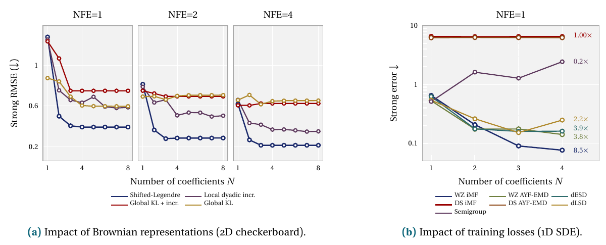
Two alternatives lose (reported, Section 3.2). Discretised Eulerian and Lagrangian losses, a small Euler-Maruyama step in place of the derivative, beat the semigroup loss on the toy and slightly lose to it at scale. The Doss-Sussmann transform, , makes the SDE an ODE in , but its derivative never involves the higher coefficients: on the 1D toy at 1 step its strong error sits near 6.5 at every (reported, Table 4).
Three changes to the map itself
The second half of the paper is a fine-tuning recipe. It starts from a pre-trained Decoupled MeanFlow model, DMF-XL/2+, which is itself distilled from SiT-XL/2+REPA. DMF turns a one-time flow model into a two-time map by feeding to the first 20 of the 28 transformer blocks and to the last 8 (reported, Appendix G.1), so at the map is the pre-trained velocity field. iSSFM adds the Brownian coefficients through a zero-initialised residual scaled by , and freezes the backbone under rank-16 LoRA adapters. On the diagonal the coefficients vanish and the network is exactly the teacher at initialisation.
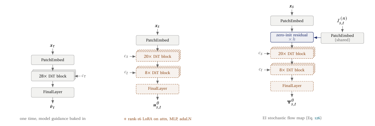
The SDE's drift is . The linear term is stiff and diverges as , and a learned map would have to integrate it on top of the teacher. The three changes:
- Exponential lift. Multiply through by . Itô's product rule gives : no linear term. The map becomes an exponentially weighted step,
- Closed-form martingale. The noise term is a time-changed Brownian motion (Dambis-Dubins-Schwarz), run on the clock of its quadratic variation. For the linear schedule that clock is as , bounded where is not (reported, Appendix B.4.1). SSFM learned a diffusion head for this term; iSSFM computes it exactly and builds the Legendre coefficients on the lifted clock, so the map's noise and the coefficients the network sees come from the same path.
- Drift matching. With the noise exact, the diagonal can regress directly onto the teacher's drift instead of onto a small Euler-Maruyama step.
The paper says the order matters: the closed-form martingale without the lift has infinite variance near , and their run of it "diverged completely into pure noise".
The training loss in the lifted state is iMF: regress onto , with the JVP's tangent along the smoothed lifted field (reported, Appendix G.2). The code matches (measured, dmf_wz_imf.py): the compound is lift_s * u - a_st * material_derivative.detach(), the target is lift_s * v_field, and the Wong-Zakai driver enters only the JVP tangent b_y = lift_s * v_field + driver_s. A comment says why: the driver "cancels in the compound identity, so the regression target stays the deterministic start field". The path information reaches the network through the material derivative, which is exactly where the semigroup loss had nothing.
The recipe (reported, Appendix G): 75% of each batch on the distillation term and 25% on the diagonal, , step at least 0.05, AdamW at , effective batch 128, 100k steps, EMA 0.9999, coefficients, one H100 NVL per run. The released checkpoint holds only what was trained (measured, safetensors header of issfm/model.safetensors): 38,571,008 float32 parameters, of which 12,003,584 are LoRA, 26,547,840 sit in a module named fixed_residual.levy_net (the coefficient pathway) and 19,584 in the coefficient embedder. The SSFM checkpoint has 41,245,968, the extra 2.67 million in its learned diffusion layer. Both load on top of the DMF-XL/2+ backbone.
Checking the ImageNet claims
All numbers in this section are FID-50k and FD-DINOv2-50k on class-conditional ImageNet-256, fine-tuned for 100k steps from the same DMF-XL/2+ (reported, Tables 1, 3 and 5). Lower is better.
| NFE | SSFM FD | + param. FD | iSSFM FD | SSFM FID | + param. FID | iSSFM FID |
|---|---|---|---|---|---|---|
| 1 | 2116.9 | 1817.6 | 994.2 | 197.11 | 184.74 | 111.61 |
| 2 | 1061.3 | 772.3 | 583.5 | 83.56 | 57.99 | 53.11 |
| 4 | 475.1 | 288.1 | 143.0 | 31.00 | 14.67 | 5.96 |
| 8 | 229.1 | 128.2 | 75.2 | 11.09 | 4.15 | 2.37 |
| 16 | 135.6 | 70.8 | 55.1 | 4.82 | 2.03 | 2.07 |
"+ param." is SSFM with all three parameterisation changes, still trained with the semigroup loss. iSSFM adds the Wong-Zakai iMF loss.
"~3x lower FD-DINOv2 than SSFM at 4 NFE"
Holds at 4 and 8 steps: 475.1 / 143.0 = 3.3 and 229.1 / 75.2 = 3.0 (reasoned). It is 2.1 at 1 step, 1.8 at 2 and 2.5 at 16. The split between the two contributions is uneven. The parameterisation alone gives 1.65 to 1.92 at 4 to 16 steps, more than the "roughly 1.5x" the paper says. The loss alone gives 2.0 at 4 steps, 1.7 at 8 and 1.3 at 16 (reasoned). At 16 steps the improved parameterisation with the old loss has the better FID, 2.03 against 2.07. The new loss matters most where steps are few, which is where it should.
The baseline needs a note. "SSFM" here is the authors' port of SSFM into the fine-tuning setting, "the most faithful replication of SSFM in our setting". The original SSFM paper trained from scratch and reported CIFAR-10 and CelebA-64 only: FID 3.49 at 4 steps on CIFAR-10, against deterministic flow maps at 3.34 (reported, SSFM Table 2). There is no head-to-head on a shared benchmark between the published SSFM and iSSFM.
"4-step iSSFM matches 16-step SSFM"
In FD-DINOv2, roughly: 143.0 against 135.6, 5% worse (reasoned). In FID, no: 5.96 against 4.82.
"~15x fewer NFE than the SiT SDE sampler at matched FD"
This one is read off a curve. The SiT-XL/2+REPA baseline is the SDE integrated by Euler-Maruyama, measured at 1, 3, 8, 17, 85, 170 and 426 steps, with FD-DINOv2 of 1288.1 at 17 steps and 88.5 at 85 (reported, Table 5). The dashed "15x" line in Figure 1 runs from iSSFM's 2-step point, 583.5, to the SiT curve between those two samples. Interpolating log-linearly between them puts SiT at 583.5 near 27 steps, about 14x (reasoned). That is a matched FD of 583.5, where FID is 53.11: an unusable sample quality. At usable quality the table gives a direct comparison: iSSFM at 8 steps (FD 75.2, FID 2.37) beats SiT at 85 (FD 88.5, FID 3.65), about 10.6x fewer steps, and SiT at 170 steps is better than any iSSFM row in FID (1.77 against 2.07).
Euler-Maruyama is also the weakest SDE sampler one could pick, and iSSFM starts from DMF-XL/2+, a deterministic few-step model whose own scores the paper does not tabulate. The limitations section says it plainly: iSSFMs "still struggle to match the performance of deterministic few-step models". What iSSFM buys over a deterministic map is not quality per step. It is a sampler whose noise you control pathwise.
Is it still strong?
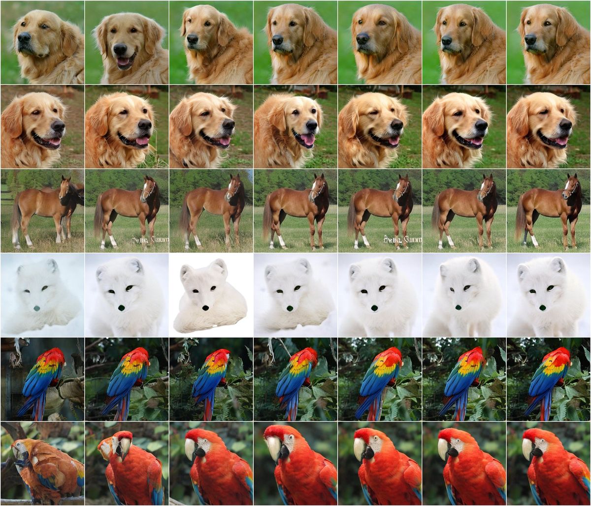
The figure above is the qualitative test. The quantitative one is Figure 5b: latent MSE of a -step rollout against the same model's 32-step rollout on the same path, over 1,000 images. Here the source and the picture disagree. The text says the semigroup-trained map "exhibits stronger pathwise consistency, at the cost of worse metrics". The plotted legend says the opposite: the lower, more consistent curve is labelled iSSFM. The LaTeX resolves it (measured, tikz/strong-consistency.tikz and its .dat): the olive curve is drawn from the column psd (semigroup) and the navy from imf, but the legend lists iSSFM first. The legend is swapped. The data say: the iMF-trained iSSFM goes from 0.956 at 1 step to 0.432 at 4 and 0.188 at 16; the semigroup map from 0.230 to 0.158 to 0.091; the weak baseline, which redraws the path every rollout, stays near 1.0 to 1.3. So iSSFM is strong, its error falls with steps where a weak map's does not, but it is about twice as far from its own 32-step answer as the semigroup map at 4 and 16 steps. The derivative loss bought sample quality with some pathwise consistency, as the text says.
The toy losses, rerun on a CPU
The paper's loss comparison is a 1D non-linear SDE, with linear from 20 to 0.1, and strong error against a 512-step Euler-Maruyama reference on 1,024 shared paths (reported, Table 4). At one step, WZ-iMF falls from 0.65 at to 0.0763 at , an 8.5x drop as coefficients are added. The semigroup loss goes the other way, 0.513 to 2.44, and at blows up at 4 and 8 steps (289 and 67,000). The discrete Eulerian loss is competitive at most step counts and best at 8. Doss-Sussmann iMF is the worst at 1 step and the best at 32 (0.00224). The win is a few-step win.
I ran two cells of that grid myself (measured, shared 4-core cloud VM, CPU only, PyTorch 2.14.1, 2 threads). The release needs Lightning and Hydra to train; I wrote a short loop that imports the repo's own Toy1DSSFMLoss, SSFM_MLP and strong-error helpers at commit cb7b92d and mirrors configs/experiment/toy1d.yaml: a 256-wide, 4-deep MLP, AdamW at , EMA 0.999, . The difference is the budget. Six authors shared the machine, so each run got 1,200 steps at batch 1,024, about 6% of the paper's 5,000 steps at 4,096, and no learning-rate scheduler. Evaluation copies the repo's callback: 1,024 paths, seed 12345, 512-step reference.
| strong error, | 1 step | 2 | 4 | 8 | 32 |
|---|---|---|---|---|---|
| WZ-iMF, my run | 5.65 | 2.70 | 1.91 | 1.54 | 1.27 |
| semigroup, my run | 6.21 | 1.73 | 0.623 | 0.508 | 0.445 |
| WZ-iMF, paper | 0.09 | 0.0466 | 0.0362 | 0.0256 | 0.0191 |
| semigroup, paper | 1.28 | 0.585 | 0.311 | 0.131 | 0.0117 |
At this budget I do not reproduce the ranking. WZ-iMF is slightly better at one step and worse from two steps on, and both are an order of magnitude or more from the paper's numbers. The 32-step column says why: it measures the diagonal, and the iMF run's diagonal loss ended at 0.32 against the semigroup run's 0.14. My reading (reasoned): the iMF compound puts a JVP-corrected target on a quarter of each batch, and in the first 1,200 steps that slowed the drift fit the whole map rests on. It is a statement about early training, not about the converged method. One full-budget cell is about 17 times the samples of mine, and the paper's grid is 36 cells; neither fit.
What holds
- The mechanism. Training the flow map of the Wong-Zakai random ODE is a sound way to get an Eulerian loss for a pathwise SDE map. The bound is standard and correctly proved, the derivative is closed-form, and the transport term makes the network read every coefficient.
- The ImageNet gain over SSFM. About 3x in FD-DINOv2 at 4 and 8 steps, roughly half from the parameterisation and half from the loss, against the authors' port of SSFM. The loss's share falls to 1.3x at 16 steps.
- The strong property. Yes, at a cost visible in the authors' own data: the iMF map is less self-consistent than the semigroup map, and the published legend says the reverse.
- The step savings against SiT. About 10x at matched quality by the table, against an Euler-Maruyama SDE sampler. The 15x is an interpolation at a quality nobody samples at.
- The toy ranking. Not reproduced in my 6%-budget runs; not refuted either.
What I find most useful is the framing: a strong stochastic flow map now trains like a deterministic one, on an ODE, with the noise turned into an input the derivative can see. The Feynman-Kac result in Section 4.3, where the map carries a particle's log-weight along its own path so resampling works at 4 steps, is something only a strong map can do, and the better reason to want one. The data-space iteration piece covers the deterministic few-step side of this family; the diffusion transformer page covers the backbone under DMF and SiT.