2026-10-17 · 20 min · physics · molecular-dynamics · flow-matching · distillation · jax · transformers
A 1:54 narrated explainer, drawn in code. Every number and picture in it is this article's own; the sources are below.
› transcript
Hi, I'm Jackstraw! Molecular dynamics crawls one femtosecond at a time. Here's how a network learns steps ten times bigger. Don't just learn the force. Learn where the molecule ends up after a big step, given the random kicks along the way. The update looks like the simplest integrator there is. But the force is averaged along the true path, not taken at the start. The velocity is averaged over the step too. And the thermal kick is sampled first and handed in. A transformer reads the atoms, their velocities, and the step size. It also reads four polynomial coefficients per atom that summarise the Brownian path over the step. Two heads predict the averaged velocity and the averaged force. One update jumps to the next state, up to ten femtoseconds later. No trajectories needed. Take a single conformer and its forces. Draw velocities at the target temperature. At a zero step, the force head must match the true force. And one big step must land where two half steps land, on the same path. A smooth polynomial summarises the grey Brownian path. From it, the flow map jumps velocity and position onto the fine path. The usual integrator: about one femtosecond per force call. The flow map: up to ten, but it needs a temperature corrector. On alanine dipeptide, that is ten times the same network as a force field, and level with classical dynamics. Learning the integral of the forces buys bigger steps. The sampler is only as good as the fit. Average over the step, hand in the noise, and train on half steps. Every source is in the full article. I'm Jackstraw. Bye!
Why read this
Hightop 30%The LFM objective derived from the SDE, the speed and transfer claims rechecked against tables and released files, and the 9M checkpoint run on CPU.
- Original analysis
- Runs on a consumer GPU
- A lasting reference
Training & RLMixed licencesResearch paper
How this was scored
- Is it new?
- 2 of 3: A real new idea, method or capability
- Can I trust it?
- 2 of 3: Measures key facts from files, code or configs
- Can I run it?
- 2 of 3: Open code or weights with real limits
- Will I understand it?
- 2 of 3: Mechanism from first principles with figures
- Can I act on it?
- 2 of 3: A concrete recipe, numbers or comparison
- Will it last?
- 2 of 3: A reference for a year or more
- Does it affect many?
- 1 of 3: A specialist community
- Only here?
- 2 of 3: A teardown or measurement few others did
Score 68 of 100, ranked 166 of 577 rated articles. Each question is answered 0–3 by hand, and a 3 is rare. How articles are scored
A machine-learned force field (MLFF) answers one question: given the atoms, what are the forces? Molecular dynamics then asks a second one a billion times: where are the atoms one femtosecond from now? The second is still answered by a hand-written integrator, at about 1 fs and one network call per step.
Langevin Flow Maps (LFMs) move the second question into the network. The paper is Langevin Flow Maps: Efficient Molecular Dynamics and Transition Path Sampling by Sam McCallum and Niklas Rindtorff (equal contribution), with Alexander Tong and James Foster, from the University of Bath and AITHYRA. Code is at sammccallum/lfm (JAX and Equinox), checkpoints and trajectories at niklastr/langevin_flow_maps, and the training set at niklastr/many_peptides_forces. Rindtorff's thread promises three things: transferable across molecular systems, transition dynamics preserved, no trajectory data required.
I read the paper and the code, pulled the released checkpoint metadata and trajectory receipts, and ran the released 9M-parameter transferable model on a CPU against Amber14 on a dipeptide it never saw. Every number below is labelled measured (I computed it from a file or a run), reported (the authors' figure, not re-run) or reasoned (my arithmetic on the other two).
The short version: the training trick is real, and the headline speedups are narrower than they read. "An order of magnitude faster than current machine-learned force fields" is the same network taking a 10x larger step. Parity with classical MD holds at 8 fs for small peptides. Large steps buy coverage of metastable states at a measurable cost in ensemble accuracy, which the authors say themselves.
Why molecular dynamics takes femtosecond steps
Molecular dynamics at constant temperature integrates Langevin dynamics. For positions , velocities , mass , friction and potential :
is Brownian motion, the thermal kicks of an implicit bath. The stationary distribution is Boltzmann, : average a long trajectory for equilibrium properties, watch it hop between basins for kinetics.
The standard integrator, BAOAB, splits the SDE into a position drift (A), a force kick (B) and an exact Ornstein-Uhlenbeck thermostat step (O), with global weak error (reported, Section 2). Bond vibrations involving hydrogen set the step near 1 fs. Conformational change takes nanoseconds to microseconds, and one microsecond at 1 fs is force calls.
An MLFF makes each call cheaper than DFT, but it is still a network evaluation per femtosecond. The thread opens on exactly this: MLFFs are "still slower than common molecular mechanics forcefields", and many are unstable in long runs for reasons accuracy alone does not explain, the forces are not enough problem.
A flow map: learn the integral, not the integrand
The alternative is to learn the solution operator itself. Fix a starting state and a realisation of the Brownian path on . The SDE is then just an ODE with a known forcing term, so the end state is a deterministic function of the two:
That is the pathwise (strong) solution map. A flow map learns for a large in one network call. The paper writes it in an Euler-Maruyama shape with learned averages (its Equation 7):
where and are the velocity and force averaged over the true path from to , both functions of and the Brownian path. As they collapse to the instantaneous velocity and force, so the same network is an ordinary force field when asked about a zero-length step. The network has two heads, mean velocity and mean force, conditioned on and on the noise.
The widget shows the difference on one particle: overdamped Langevin dynamics in a double well at , friction 1. One Brownian path, drawn at a fine step of 0.002 for 1,000 time units, is reused everywhere. The fine Euler-Maruyama run is the reference. The exact flow map at step is that reference read every , computed by brute force: exact by construction, at evaluations per step, where an LFM would pay one. Euler at h gets the same path but sees only the force at the start of each step and the summed increment.
What it shows (measured, in-browser, seeded): the reference makes 40 well-to-well transitions; the exact map counts 38 at every step from 0.01 to 0.4, missing two brief recrossings between samples. Euler matches at , counts 46 at , and at , inside the linear stability limit , runs 792 time units before a large kick throws it past the far wall. At 0.2 it lasts 26. The first-step readout shows why: at the force is exactly zero, so Euler's drift is zero, while the force averaged along the true path is not. Learning that average is the job.
Telling the network about the noise
depends on the whole path on , not just its endpoint: a kick early in the step and one late in it end in different places. The paper summarises the path by projecting it onto shifted Legendre polynomials (Foster, Lyons and Oberhauser, 2020). The coefficients have two properties that make the method work (reported, Section 3.2 and Appendix A.1):
- They are independent Gaussians, , so they can be sampled directly without building a fine path. is the increment ; the higher ones describe how the path bends away from the straight line.
- Coefficients on and combine into coefficients on by a closed-form linear rule (the Chen relation). For degree 1, .
Both are in langevin_flow_maps/brownian.py (measured): sample draws std = sqrt((t - s) / (2n + 1)), and _chen_coefficients builds the combination matrix in exact rationals, with a comment that the alternating sum "cancel[s] catastrophically in floating point" otherwise. The model uses degree 4, so each atom gets four 3-vectors of noise information, embedded alongside the step size, velocity and mass and injected into every transformer block through adaptive layer norm (reported, Appendix B; Table 4 lists 6 blocks, 8 heads, hidden size 256).
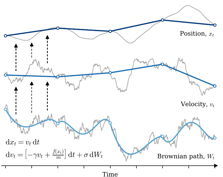
On ethanol, both integration error and structure error fall as the degree rises, with the largest drop from increment-only to the first higher coefficient (reported, Figure 9). On the released transferable model, telling an 8 fs step only the increment makes it about four times worse (measured, below).
Training without trajectories
How do you supervise a map from start state to end state when you have no trajectories, only a pile of single conformers with forces? The paper's Proposition 3.1, inherited from the authors' earlier Strong Stochastic Flow Maps work, says a candidate map is the true solution map if and only if two things hold:
- Boundary condition. At the heads return the true velocity and the true force.
- Semigroup property. One step of equals two steps of with the matching halves of the same Brownian path: for .
Each becomes a loss. The first is ordinary force matching. The second is self-distillation: sample a start state, a step and two half-interval sets of Brownian coefficients; run the EMA "teacher" copy twice at ; Chen-combine the coefficients; ask the student to land in the same place in one step, with the error divided by and no gradient through the teacher. It is the shortcut model trick from image generation, applied to a physical SDE with the noise made explicit; the flow maps in data-space iteration and the one-step heads in Pocket TTS with drifting are the same family.
The data requirement falls out. The dynamics are time-homogeneous, so no sample needs a timestamp: positions and forces come from any equilibrium dataset, velocities from Maxwell-Boltzmann. The code matches (measured, experiments/train.py): sample_velocities draws Gaussian velocities from kB * T / m, a quarter of each batch (eta=0.25) goes to matching and the rest to distillation, step sizes are log-uniform between 0.01 and 10 fs, the EMA decay is 0.99, and the loss is eta * matching + (1 - eta) * distillation. "No trajectory data" holds for training. Evaluation still compares against long reference MD, as it must.
Two things differ from the paper's text. Its transferable section claims "the same single-molecule architecture and training setup" (Adam, cosine schedule), but experiments/train_transferable.py uses a Muon variant with a warmup-stable-decay schedule, and the released 9M checkpoint's metadata says "optimizer": "kimi_muonw_adamw" (measured). And the transferable labels are not quantum: the dataset card says every frame carries "AMBER14 + OBC1 implicit-solvent potential energies and forces" (measured). MD17 runs learn DFT forces; the transferable model learns to integrate a classical force field faster.
Is it still a Boltzmann sampler?
Not by construction. An LFM is a learned approximation with no Metropolis correction, so residual error in the heads enters every step. The paper says so in Appendix C.3.1: the remaining bias "over many steps can introduce a bias to the kinetic temperature", fixed at inference by a temperature corrector that rescales the noise term so the mean kinetic energy hits per element.
Why not a learned Hamiltonian map plus a thermostat? Because the deterministic and stochastic parts do not commute, so even a perfect Hamiltonian map alternated with an O step biases transition dynamics at large steps (reported, Section 2). Learning the whole stochastic map removes that bias. It does not remove fitting error.
How much the corrector carries surprised me. I ran the released 9M checkpoint (9M_500A, 9,221,191 parameters, measured) on the AA dipeptide, one of the nine held-out test peptides, at 8 fs for 16 trajectories, once with the corrector and once without. Uncorrected, the mean kinetic temperature climbs from 310 K to about 450 K within a picosecond and sits there; over the second half it averages 457 K (measured). With the corrector, the potential energies of the frames, scored by Amber14/OBC1 in OpenMM, land close to the released 1 µs Amber14 reference trajectory: mean -455.9 versus -459.0 kJ/mol, 1D Wasserstein-2 distance 4.3 kJ/mol against a sampling floor of 0.2 (measured). Without it, W2 is 42.7 kJ/mol. A 2 fs corrected run was no better than 8 fs here (W2 5.0), but it covers only 4 ps per trajectory, so I would not read much into that.
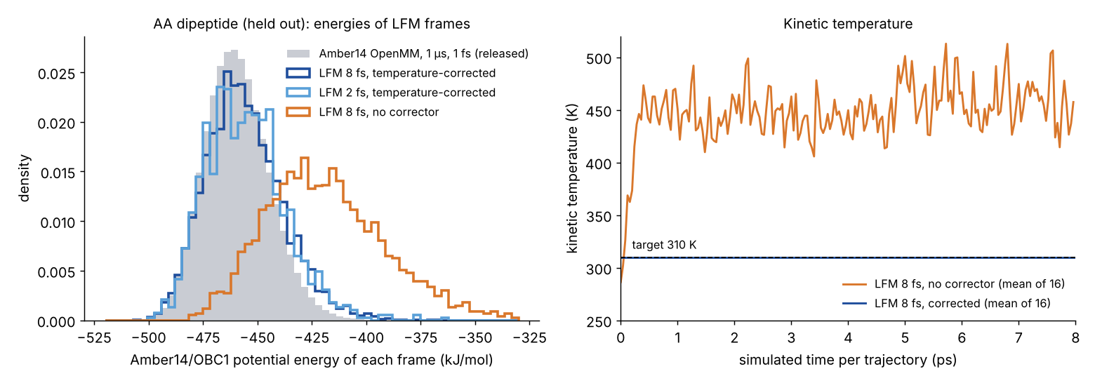
One detail of the corrector matters if you use it (measured, flow_map.py): TemperatureCorrectedFlowMap.batch_step averages kinetic energy across the batch before solving for the noise scale. It constrains the ensemble mean, not each trajectory. In my corrected 8 fs batch the batch mean is pinned at 310 K, while one trajectory touched 574 K. Run with a batch of one and it becomes a per-trajectory thermostat, which is a different algorithm.
Checking the claims
"An order of magnitude faster than current machine-learned force fields"
The evidence is alanine dipeptide, Figure 5 of the paper. Throughput on one RTX A6000 is 1,726 ps per minute for the LFM, 173 for the MLFF and 1,523 for classical MD (reported).
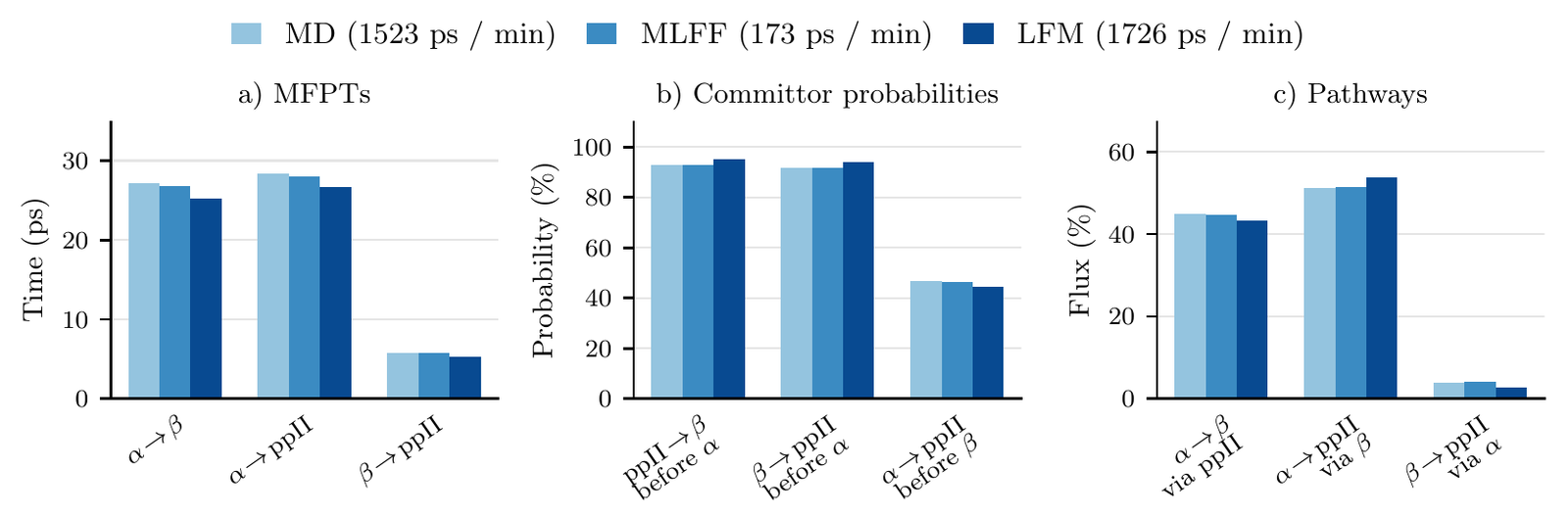
Read the setup before the ratio. The "MLFF" is the LFM's own force head queried at and integrated with BAOAB at 1 fs; the LFM runs at 10 fs (reported, Appendix C.2). Same network, ten times the step: 1,726 / 173 = 9.98 (reasoned). That is the honest version of the claim. It is not a comparison against a separately trained MLFF such as MACE or NequIP. Against classical MD (Amber99SB-ILDN in OpenMM at 1 fs), 1,726 / 1,523 is 1.13x (reasoned), and that classical engine was running a 22-atom molecule on a GPU, where it is mostly launch overhead.
The kinetics hold up on this system. The LFM's mean first passage times sit a little below the MD reference, by about 2 ps on α→β read off the bars, with committors and pathway fluxes within a few points (reported, Figure 5). For a single small molecule with a dedicated model, that is a good result.
Parity with classical MD
For the transferable model, Figure 14 is the throughput plot, on one RTX PRO 6000 Blackwell.
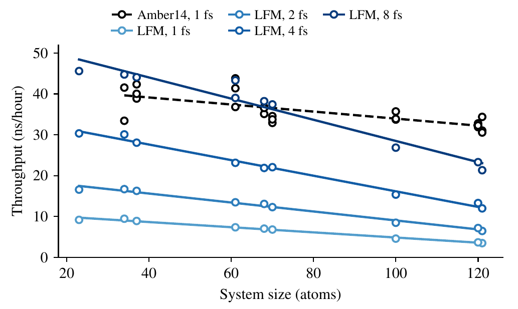
At 8 fs the LFM matches Amber14 up to roughly 70 atoms and falls behind above it; at 120 atoms it is around 23 ns/hour against 32 (reported, read off the figure). The pairwise-distance embedding grows with the square of the atom count (the paper's limitations section). Rindtorff's thread is plain about it: "we're only reaching simulation time/wall clock time parity with classical molecular mechanics for large steps and relatively small molecular systems." And in the replies, the biggest systems simulated so far are "at the ca. 200 atom mark", with explicit solvent at roughly 1,000 atoms still out of reach.
The released receipts agree on the order of magnitude. The OpenMM run for AA records 1,122 ns/day, which is 46.8 ns/hour, and the learned-force BAOAB baseline on the same peptide records 9.88 ns/hour at 1 fs (measured, results.json in each run; the GPU is not recorded there).
On a CPU it is worse for the network. On two cores of a shared 4-core VM, one LFM step on the 23-atom AA costs 27.7 ms, a zero-step force query 25.2 ms, and a batch of 16 trajectories 314 ms (measured). OpenMM's CPU platform runs AA at 3,113 steps per second, 11.2 ns/hour (measured). At 8 fs the LFM manages 1.04 ns/hour for one trajectory and 1.47 summed over 16 (reasoned). Classical MD wins by 8 to 11x; the machine was shared, so read these as orders of magnitude.
Stability
"Forces are not enough" is about MLFF simulations falling apart. The released data has one example of that on the baseline, not the LFM: the learned-force BAOAB rollout for the octapeptide PGESTAES stopped at 48.977 ns with a kinetic temperature of 743.8 K and a 20.7 Å bond (measured, failure.json). The sampling table only uses the first 10 ns of each baseline run, so the failure does not touch Table 3, and the release notes say so.
The LFM's own forward trajectories are "not included in this release" (model card), so I cannot check their long-run stability. My runs were short: 2,000 steps (16 ps) per trajectory at 8 fs and 4 ps at 2 fs, all finite, with the longest bond in any saved frame at 1.65 Å (1.70 Å uncorrected), well inside the 3 Å blow-up threshold the authors' own rollout scripts use (measured). No early blow-up; nothing more.
Transition dynamics and transfer
The transferable model is a 9M-parameter LFM trained on Many Peptides Forces: 434M frames in 5,000 shards per the dataset's completion.json (measured), peptides of length 2 to 8, Amber14/OBC1 labels at 310 K. The released checkpoint's metadata lists 20,615 training sequences, 497,814 optimizer steps and about 4.44 billion atom exposures, which is the "480 atoms per parameter" budget (measured). Table 3 evaluates on nine held-out peptides, three each of length 2, 4 and 8, with function evaluations per run.
Two kinds of metric pull in opposite directions (reported, Table 3):
| Length | Metric | LFM 8 fs | LFM 4 fs | LFM 1 fs | Amber14 1 fs |
|---|---|---|---|---|---|
| 2AA | energy W2 | 3.64 | 2.73 | 1.20 | 0.30 |
| 2AA | state occupancy TV | 0.13 | 0.07 | 0.21 | 0.15 |
| 4AA | energy W2 | 11.75 | 8.76 | 5.08 | 1.04 |
| 4AA | transition TV | 0.19 | 0.18 | 0.43 | 0.27 |
| 8AA | energy W2 | 25.91 | 20.90 | 11.45 | 4.04 |
| 8AA | state occupancy TV | 0.03 | 0.03 | 0.05 | 0.07 |
Energy and torsion distributions get worse as the step grows; at 8AA the 8 fs energy W2 is 6.4x the Amber baseline's (reasoned). State occupancy and transition probabilities get better than Amber14 at large steps. The reason is in the setup: at a matched evaluations, 8 fs steps cover 80 ns while 1 fs covers 10 ns (reasoned). Rare basins get visited because more physical time elapsed. The thread names the trade fairly, "a knob to trade mode coverage for energetic fidelity", but "transition dynamics are preserved" leans on it: the large-step model explores faster, not more accurately per nanosecond. At 8AA the transition-probability TV is 0.45 to 0.49 for every row, Amber included, which says the metric is saturated there.
The most interesting result is Figure 13. On the held-out octapeptide ANKSMIEA the LFM visits a basin that the reference Many Peptides MD never reached. The authors seeded three Amber14 runs in it and they stayed for 11.5, 6.8 and 15.8 ns (reported; the three 100 ns validation runs are in the release).
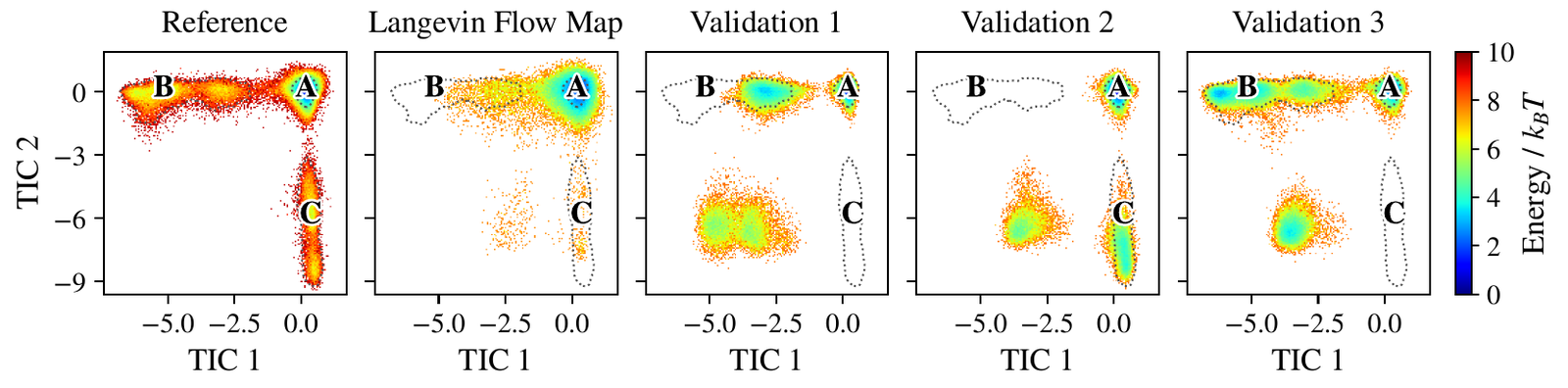
That is the workflow the authors propose: explore with big LFM steps, confirm and measure with small ones.
What I ran
| What | Result | Label |
|---|---|---|
Released 9M_500A parameters | 9,221,191 | measured |
| Force error vs Amber14 at h = 0, one AA frame | RMSE 3.76 meV/Å (paper's mean over 92 test systems: 6.61) | measured / reported |
| One 8 fs step vs 64 steps of 0.125 fs, same Brownian path, 16 AA states | position RMSE 0.0038 Å against a 0.133 Å displacement | measured |
| Same 8 fs step told only the increment | 0.0163 Å, about 4x worse | measured |
| Kinetic temperature, 8 fs, no corrector | 457 K against a 310 K target | measured |
| Amber14 energy W2 vs 1 µs reference, 8 fs corrected | 4.3 kJ/mol (uncorrected 42.7) | measured |
| CPU throughput, 2 threads, AA | OpenMM 11.2 ns/hour; LFM 8 fs about 1 to 1.5 ns/hour | measured / reasoned |
The consistency rows measure the network against itself at finer steps, which is what the semigroup loss trains: the map composes cleanly, which is not the same as matching Amber14. The energy row is the comparison against physics. Setup: Python 3.12, JAX on CPU, the repo from a shallow clone, OpenMM 8.6, AA's released initial.pdb as the start.
Where it breaks
- System size. The pairwise embedding is quadratic in atoms. Parity ends around 70; nothing over about 200 has run.
- Bias. The ensemble drifts as the step grows, with no accept/reject step to pull it back; the corrector is not optional.
- Labels. The transferable model learns Amber14. QM accuracy is the per-molecule MD17 story.
- Direct forces. The force head is not an energy gradient, so it is not conservative even at .
- Licence. The GitHub repository has no licence file (measured, commit
ebaadac); the checkpoints are MIT and the dataset CC-BY-4.0.
- branch
- main
- tests
- none found
- source
- 95.9 kB
- commit date
- 2026-10-06
by size of tracked source at this commit, file counts in brackets; docs, data and vendored trees excluded
local clone, 2026-10-17 at ebaadac — branch, commit, commitDate, fileCount, hasTests, languages, shallow
shallow clone: counts describe the pinned tree, not the history
Verdict
The idea is the part to remember: in molecular dynamics the force field was never the whole cost. The step size is a second factor of ten, and it can be learned from the same single-conformer data used to fit the forces, by making the network consistent with itself over half steps while handing it the Brownian path. No trajectories, no new labels.
The numbers say "promising", not "faster MD today": the 10x is a step ratio, parity with classical MD holds for small peptides, and the map needs a thermostat patch to hold its temperature. For exploring small systems, where coverage is the bottleneck and you relax with small steps afterwards, it is already useful.
Related reading on this site: data-space iteration and CSFM for flow maps and flow matching in image generation, Pocket TTS with drifting for one-step self-distillation objectives, and Extropic Z1T for hardware built around sampling.