2026-10-02 · 13 min · self-supervised-learning · representation-learning · vision-transformers · pretraining · attention · explainer
A masked self-supervised image model has a cheap way to win that no one wants it to find. If the task is "look at the parts of the image I left you and predict the parts I hid," a vision transformer can go a long way on position and local texture alone: the patch above a hidden one is usually a decent guess for it, and the grid of fixed positional embeddings tells the model exactly where everything sits. The features it learns are good enough to reconstruct, and worse than they look for anything that needs to know what is in the image rather than where.
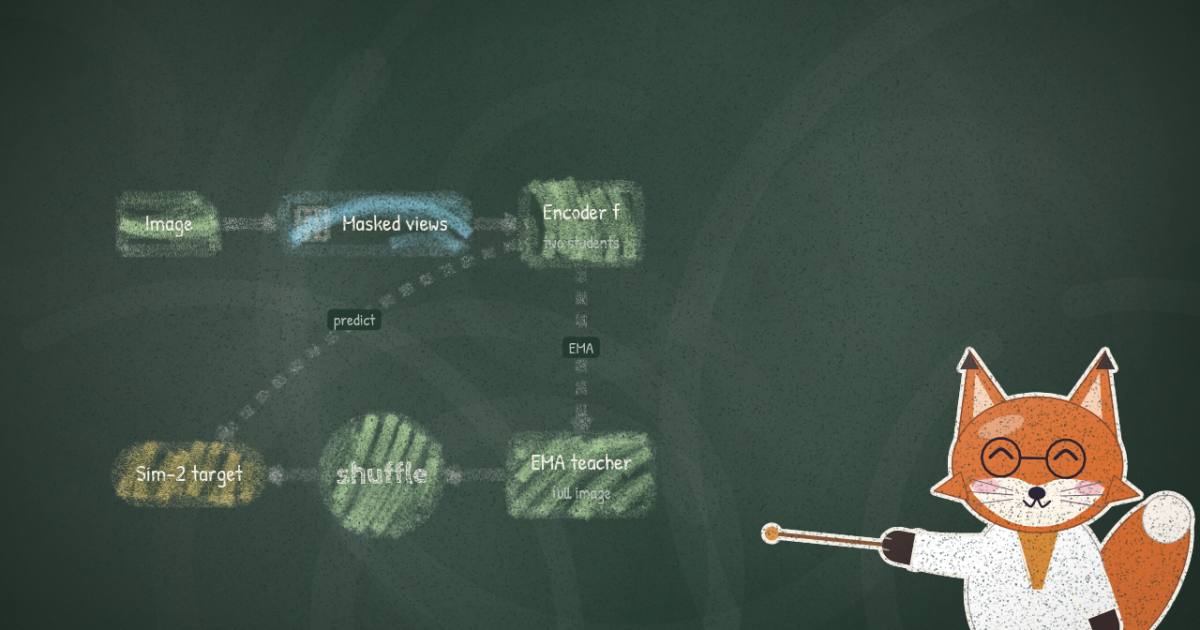
SiamJEPA (Makoto Yamada, Okinawa Institute of Science and Technology; arXiv 2607.04044, single author) is a self-supervised representation-learning method in the I-JEPA lineage whose one genuinely new part is a blunt instrument aimed straight at that shortcut. It is called the Random Shuffle Teacher (RST): before the model computes its prediction target, it randomly permutes the teacher's patch tokens — after their true positional embedding has already been added. The correspondence between a position and the content that lives there is destroyed, and a model that was relying on "the patch at slot 14 is usually object-ish" suddenly cannot, because slot 14 now holds some other patch, and a different one on every forward pass.
I read the paper and cloned the training code to check two things: that the method is what the abstract says it is, and that the code implements it. Both hold. What does not hold cleanly yet is the leaderboard — the repository's own README (September 2026) says the headline ImageNet numbers were measured before a shuffling bug was fixed and will be revised. So this is a piece about the mechanism and why it is interesting, with the accuracy deltas marked provisional throughout.
What JEPA predicts, and why that gives semantic features
The Joint-Embedding Predictive Architecture family starts from a simple decision about what to predict. Masked autoencoders reconstruct pixels: hide 75% of the patches, make the model paint them back in, and the loss is pixel error. That admits no collapsed solution — you cannot reconstruct a photograph by outputting a constant — but it spends the model's capacity on texture and high-frequency detail that a downstream classifier does not care about.
I-JEPA changed the target. Instead of predicting pixels, it predicts the latent representation of the masked region, as produced by a target encoder looking at the full image. The loss lives in embedding space, not pixel space, so the model is never asked to reproduce the exact texture of a hidden patch — only what a good encoder would say about it. That nudges the features toward semantics: to predict the target encoder's embedding of a hidden region, you have to predict its content at the level the encoder abstracts to, not its pixels.
SiamJEPA keeps that core — predict the teacher's latent embeddings of masked patches, measured in latent space — and rebuilds the rest of the architecture around a Siamese pair of students.
Two students, one teacher, two losses
Here is the method as the code runs it (models_siamjepa.py, forward()). Each image is masked twice,
into two disjoint sets of visible patches, and both masked views go through the same encoder
— that is the Siamese pair (the paper's and ). A
separate EMA teacher — an exponential moving average of the student's weights,
updated with a momentum schedule — sees the full, unmasked image and
produces the prediction targets . The teacher never receives a gradient; it is a slow,
stable copy of the student the student chases.
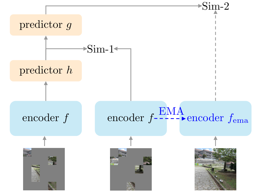
Two loss terms hang off that diagram, and the paper names them Sim-1 and Sim-2.
Sim-2 is the JEPA prediction. A shallow predictor (a single cross-attention block — the ViT-Base
config uses decoder_depth=1) takes a student's visible tokens plus mask tokens and predicts the teacher's
representation at the hidden slots. The loss is a cosine distance, , averaged
over the patches masked in both views. A detail worth stating, because I only know it from reading the
code: the paper writes this term as an MSE, and on the L2-normalized vectors the code actually feeds it,
is the squared Euclidean distance — the cosine form is the normalized MSE, not a different
loss (measured, models_siamjepa.py lines 761-774).
Sim-1 aligns the two students. This is the part that makes SiamJEPA "Siamese" rather than just a
single-student JEPA, and it is a KL term, not a feature-matching loss. Each student's [cls] summary feeds
a small stochastic head that produces a categorical latent (the DreamerV2-style 32 × 32
discrete code): a posterior conditioned on both views and a prior conditioned on one. Sim-1 is the KL
between posterior and prior, symmetrized across the two students, with KL-balancing (0.2) and a free-bit
floor (0.1) so the term cannot be driven to zero. The full objective is
with as the default (reported, paper; --kl_scale 0.01). The "JEPA-like"
baseline the paper compares against is the same architecture with — the
Siamese alignment turned nearly off, leaving essentially a single-student JEPA.
The paper frames all of this as a JEPA instantiation of PhiNet, Yamada's earlier brain-inspired representation-learning model: a predictive, Siamese, EMA-teacher architecture motivated by cortical learning rather than by a benchmark. That framing is why the interesting claim here is not "it is more accurate" but "look what the representations become."
The Random Shuffle Teacher
Now the one new idea. In the teacher's forward pass (forward_encoder), the positional embedding is added
to the patch tokens first. Then, if --shuffle_teacher is set, the tokens are randomly permuted and run
through the transformer in that scrambled order:
# models_siamjepa.py, forward_encoder()
x = x + self.pos_embed[:, 1:, :]        # true grid position added FIRST
if self.shuffle_teacher:
    x, _, _ = self.random_masking(x, mask_ratio=0.0)   # keep all tokens, random order
# ... transformer blocks, norm ...
The target the student is scored against is the teacher's token sitting at slot . With the ordinary ordered teacher, slot always carries the representation of patch — so a student can minimize Sim-2 with a fixed position-to-content map, which is exactly the spatial shortcut. With RST on, slot holds a different patch's representation, re-randomized every forward pass. There is no stable position-to-content map to learn. The only way to predict the token that will land at slot is for the student's own tokens to be recognizable by what object-part they are, independent of where they sit.
The widget below is that argument made concrete. Pick a patch; toggle the teacher between ordered and shuffled; in shuffled mode, draw a new sample and watch the target move.
target at slot 14: teacher is showing object centre from patch 9 — a different patch than the one at slot 14.
This sample happened to land matching content here, but that will not hold next sample. No stable position-to-content map exists: the target at slot 14 changes every forward pass. The only way to predict it is for each token to be recognisable by what it is — object-level semantics, not position.
probe of a frozen token’s own grid position, chance 0.51% (paper, Table 3; pre-fix RST, provisional)
Note what shuffling does and does not do. It preserves the multiset of patch contents — the teacher still encodes every patch of the full image — and destroys only the correspondence between position and content. That is why it pushes toward position-invariant, semantic tokens specifically, rather than just adding noise. Yamada's own framing of the result, from the thread announcing the work, is that "predicting randomly shuffled teacher patches accurately is hard, so each patch token comes to hold a semantic representation of the whole object, not just position or local information."
Is the shuffle doing it alone? No — and the paper says so
The honest version of this story has a wrinkle the abstract is careful about: the semantic bias "arises from the interaction between RST and the Siamese objective rather than from shuffling alone." The cleanest evidence is a probe the paper runs directly on the question — can you decode a frozen patch token's original grid position (1 of 196, chance ) from the token alone?
Without RST, a frozen patch token is almost perfectly position-decodable: 94.3% top-1 (reported, paper
Table 3; provisional). Turn RST on and that collapses to 18.7% (reported, paper Table 3; provisional)
— the tokens have mostly stopped carrying their own address. And the ImageNet linear-probe accuracy of those
same encoders goes the other way: 65.13% → 70.71% on the student branch over the same comparison. Less
position information in each token, more class-discriminative information. That is the mechanism, measured.
It is also where the numbers need their asterisk. These are pre-fix RST runs, so the exact 94.3 and 18.7
will move; the direction — position decodability crashes, class information rises — is the robust claim and
the point of the whole design. The RST run on its own reaches 71.13% linear probe at 400 epochs, which is
below the 72.9% I-JEPA reference: shuffling buys semantic tokens but pays in spatial precision, and raw
accuracy wants some spatial structure back.
That is what the semantic-to-spatial curriculum is for, and it is refreshingly unclever: two ordinary
pretraining runs, not a special mode. Train with --shuffle_teacher first (say 200 epochs), then continue
from that checkpoint with shuffling off (--init_checkpoint), to restore spatial correspondence on top of
the semantic tokens RST built. The curriculum checkpoint is the one that reaches the headline number.
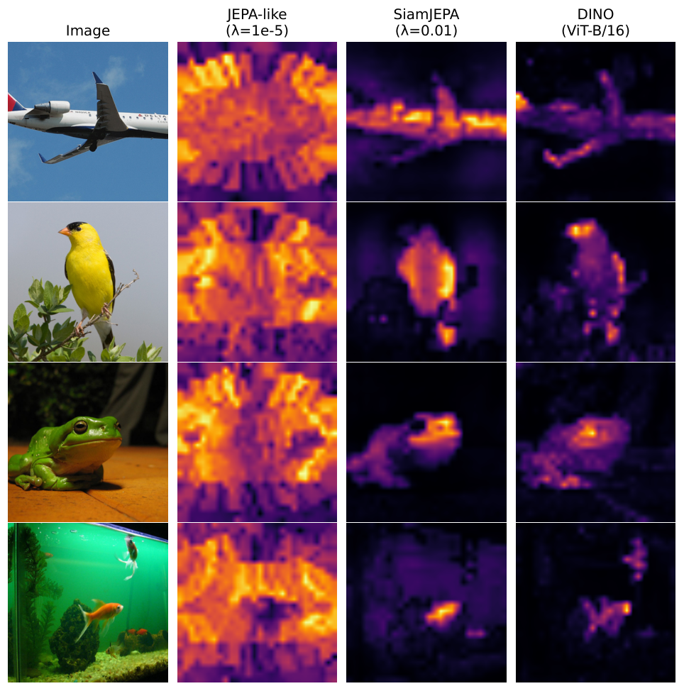
The attention maps are the other half of the same observation. With the Siamese term nearly off, last-block
[CLS] attention is a diffuse grid — attending to position, more or less uniformly. Turn it up to 0.01
and the attention snaps onto the foreground object, qualitatively like DINO.
Yamada notes in the thread that tuning the mask ratio and weight decay sharpens this further. For a
representation-learning method, an attention map that finds the object without ever being told where it is
is a more interesting result than a point of linear-probe accuracy.
The numbers, and exactly how provisional they are
With that framing, here is the leaderboard the paper reports, all of it pre-fix and provisional.
| Method | Epochs | ImageNet linear probe |
|---|---|---|
| MAE (400 ep) | 400 | 61.9% |
| I-JEPA | 600 | 72.9% |
| DSeq-JEPA | 600 | 73.5% |
| SiamJEPA + RST curriculum (12th-layer probe) | 450 | 73.3% |
| SiamJEPA + RST curriculum (I-JEPA probe protocol) | 450 | 74.2% |
The two SiamJEPA rows are the same checkpoint evaluated two ways (reported, paper Table 1; provisional).
73.3% is the standard last-layer linear probe; 74.2% is the same weights scored under I-JEPA's own
evaluation protocol (average-pooled features concatenated across four layers, best of a probe-head grid),
which is the apples-to-apples comparison against the 72.9% and 73.5% I-JEPA/DSeq-JEPA figures (those two
are reported from their own papers at 600 epochs). So the provisional claim is: a simpler masking strategy,
fewer epochs, a point or so ahead — if it survives the re-run.
Two things keep me honest about that "if." First, at matched final settings the Siamese term without RST
does not beat the JEPA-like baseline: SiamJEPA at , weight decay 0.1 scores
65.18% versus the JEPA-like 68.30% (reported, paper; provisional). The win is specific to the RST
curriculum path, not to adding a second student per se — the paper's own claim for the plain Siamese term is
narrower, that it regularizes the objective and accelerates early-stage learning. Second, the arXiv v3
(dated 2026-09-27) already contains a section analyzing the pre-fix RST checkpoint after the fix, and finds
a pre-fix training instability at that no longer appears post-fix. The
author is clearly mid-revision; the mechanism survives the fix, the exact cells are in motion.
A few practical notes from the repo, since the site cares about what actually ships. There are no released
checkpoints — the repository is training and evaluation code only, so every number here is the author's, not
something I could re-probe (measured: cloned repo, git clone --depth 1; no weights present). Pretraining is
siamjepa_vit_base_patch16 only (the large and huge variants are stubs), on 4 × H100, batch 512 with
4-step accumulation. And the license is per-file: the MAE-derived utilities are Apache 2.0, but the core
model, training and evaluation files (models_siamjepa.py, main_pretrain_siamjepa.py, and friends) are
CC BY-NC 4.0 — non-commercial (measured, LICENSE and file headers). If you want to build a product on
this, that clause is the first thing to read, not the last.
What to take away
Strip the provisional leaderboard and SiamJEPA is a clean idea about inductive bias. A JEPA already predicts in latent space, which buys semantics over a pixel model. Shuffling the teacher's targets removes the one remaining shortcut — position — and forces each token to carry object-level content, because a scrambled target is unpredictable any other way. The Siamese KL term is what turns that pressure into object-centric attention rather than noise, and a two-stage curriculum hands back the spatial precision that pure shuffling gives up. You can watch all three effects in the paper's own probes: position decodability falling, class information rising, attention finding the object.
The accuracy claim will land where it lands after the re-run. The design — predict a deliberately
position-scrambled target to make representations say what instead of where — is the part worth keeping,
and the code to check it is a git clone away.
For more on predictive self-supervised learning without the usual target-network machinery, see
LeVJEPA. For how [CLS]-to-patch attention is computed and why it localizes, see
how transformers' attention works and
the differential transformer. For vision transformers under a tight
budget, see ViT compression for plant disease, and for the
contrastive-vs-predictive framing in a multimodal encoder, SigLIP 2 on Core ML.