2026-09-26 · 22 min · explainer · interpretability · llm · benchmarks · evaluation

Matryoshka Attribution (MAttr) is a way to ask a trained network which of its parts produce a behaviour. It learns one number per part (an attention head, an MLP neuron, an SAE feature, an edge between two of them) by gradient descent, and the sorted numbers are the answer. The trick is in how it trains: every step draws a fresh budget , keeps a soft "top-" set of parts, patches the rest, and asks the output to survive. Because the soft top- masks for different budgets nest inside each other, one training run gives you a circuit at every size.
The launch post by Aryaman Arora says MAttr is "#1 on the Mechanistic Interpretability Benchmark by a wide margin (2.9× the runner up)". That holds, on one metric. I read the paper, the code and the live leaderboard to find out which metric, and what the other one says.
Attribution is a ranking problem
Circuit discovery starts from a behaviour and a counterfactual. Take indirect object identification (IOI): "When Mary and John went to the store, John gave a drink to" should continue with "Mary". The base input is that sentence. The source input swaps the names so the right answer changes. The behaviour is measured as a logit difference: the base answer's logit minus the source answer's logit.
Now pick a basis: the set of parts you will attribute to. It might be every attention head and MLP block (MIB's node level), every edge between them (edge level), every MLP neuron at every token, or every SAE feature. An interchange intervention on one part replaces its activation on the base run with its activation on the source run. If the logit difference collapses, that part mattered.
A circuit of size is a set of parts that you keep at their base values while every other part is patched to its source value. Its faithfulness is how much of the behaviour survives:
where is the logit difference, the model with only the circuit kept, the full model and the model with everything patched. means the circuit reproduces the full model's logit difference; means it recovers nothing.
Nobody knows the right in advance, so the Mechanistic Interpretability Benchmark (MIB, Mueller et al., 2025) does not ask for a circuit. It asks for a score per part, sorts it, and evaluates the top- circuit at a grid of sizes, from 0.1% of the parts to 100%. Two numbers come out of that curve. CPR is the area under ; higher is better. CMD is the area between and 1; zero is best. An attribution method is, in this framing, a function from a model and a dataset to a ranking.
Three families, three failure modes
Activation patching
The exact way to score a part is to patch it and look. One forward pass per part. On MIB's node level that is the IntInv baseline, which the paper counts at 63k to 423k forward passes per task (reported, Figure 2). It answers one question exactly: what does this part do alone? When parts interact, that is the wrong question. If three heads each carry the same signal, patching any one of them changes nothing, so each scores zero. The complete answer needs interventions on sets, and there are of those. On MIB's node-level test set IntInv scores a CPR of 1.14, below IG with 10 or 30 steps, expected gradients, GIM and AttnLRP, which score 1.28 to 1.31 (reported).
Attribution patching, EAP and EAP-IG
Attribution patching replaces the patch with its first-order Taylor term. For part :
One forward and one backward pass score every part at once. Edge attribution patching (EAP) applies the same estimate to edges. The cost is correctness wherever the model curves between and . A part feeding a saturated nonlinearity (a softmax that has already committed, a tanh near 1) has a tiny gradient at the clean run and a large effect when patched; the AtP* paper catalogues this failure for attention. EAP-IG (Hanna et al., 2024) replaces the single gradient with integrated gradients: average the gradient over a path from source to base, which fixes saturation. It keeps a quieter problem. IG is complete, so the credit of a redundant path is split between its copies, and each copy looks smaller than the path it can carry alone.
Learned masks
The third family trains the answer. Put a gate between 0 and 1 on every part, optimise the task loss plus a sparsity penalty, and read off which gates stay open. Subnetwork probing and Edge Pruning (Bhaskar et al., 2024) are the standard forms, usually with a hard-concrete relaxation and an L0 penalty. Masks see interactions, because the loss is computed with many parts patched at once. They have two costs. The sparsity coefficient and the gradient estimator need tuning and can be unstable. And one run gives one circuit at one size, so a curve over sizes means a sweep. The paper's DBM and Node Pruning sweeps cost about 50× as much as MAttr (reported).
A toy where the answer is known
To see these failure modes without a GPU, I built a 12-part toy with one output and wrote all four scorers against it. The widget computes everything live, including 200 MAttr training steps. The parts:
- L1, L2: linear paths with weights 1.2 and 0.7.
- S: a saturated unit, . At the base value its gradient is 0.074; patching it removes 2.49 of the output.
- R1, R2, R3: redundant backups feeding a soft OR, . Any one of them carries the path: R1 alone restores all of it, R2 or R3 alone 90% or 80%.
- N: a suppressor with weight −1. Keeping it lowers the output.
- X1–X5: noise, with weights no larger than 0.15 in magnitude.
Every part has base value 1 (R2 and R3 have 0.9 and 0.8) and source value 0. The "all linear" switch replaces the tanh and the OR with straight lines. The "match the model" switch changes MAttr's loss; more on that below.
| method | area ↑ | gap to 1 ↓ | passes to score all |
|---|---|---|---|
| patching | 0.935 | 0.217 | 13 forward |
| linear | 0.820 | 0.332 | 1 fwd + 1 bwd |
| IG | 1.027 | 0.179 | 16 fwd + 16 bwd |
| MAttr | 1.042 | 0.185 | 200 fwd + 200 bwd |
| brute force | — | — | 4,096 forward |
Twelve components, one output. S sits in a saturated tanh, so its gradient at the clean run is nearly zero although patching it removes 2.49 of the output. R1–R3 feed a soft OR: any one of them carries most of the path, so patching a single one costs 0.04 of the output at most. N pushes against the behaviour. Each row is one method’s ranking; the first k chips are kept at their base values and the rest are patched to the source, and f(k) is how much of the full output survives. “Area” is the mean f over k = 1…12 (a CPR analogue on a linear grid) and “gap” the mean |1 − f| (a CMD analogue). Switch the loss to “match the model” and watch N move up the MAttr ranking: area falls and the gap shrinks.
What the widget shows, with numbers measured on the toy in nonlinear mode:
- Attribution patching misses S. Its gradient score is 0.074, below two of the noise parts, so S enters its ranking fifth. At its circuit is L1 and L2, with .
- Activation patching misses the backups. Patching R1 alone costs 0.04 of the output and R2 or R3 alone cost nothing, because the other two cover. The R parts land seventh, ninth and tenth. At its circuit is S and L1, with .
- IG fixes S and splits the OR. It scores S at 2.49 but gives the backups 0.78, 0.66 and 0.56, so at it also picks S and L1 ().
- MAttr keeps one backup and drops the other two. Its ranking starts R1, S, L1, L2 and puts R2 and R3 ninth and tenth, below most of the noise, because once R1 is kept they add nothing. At it keeps R1 and S, , which is the best of all 66 pairs. It matches the brute-force best at every except , where it keeps R1 () and the best single part is S (). The soft relaxation optimises an average over budgets, not each budget.
Switch to "all linear" and all four rankings coincide: a first-order method is exact on a linear function, and MAttr learns the same order. Everything interesting about attribution happens in the curvature.
What Matryoshka Attribution optimises
MAttr is a learned mask with two changes: a sigmoid top- parametrisation, and a budget that changes every step. The paper's overview figure shows one training step.
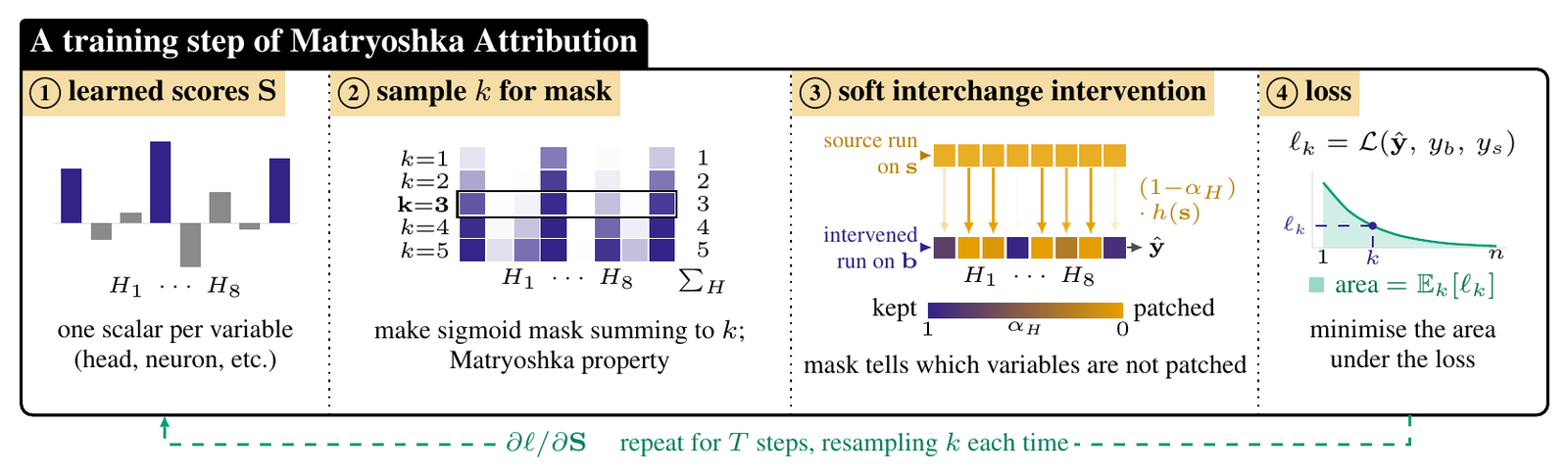
One score per part. The only trainable parameters are a vector with one entry per part in the basis, initialised to zero. The model is frozen.
A sigmoid top- mask. For a budget , the keep weight of part is , where the constant is found by bisection so that the weights sum to exactly . This operator comes from Wijk et al. (2025). The repo's scripts also divide by a temperature, by default (--T in eval_mib.py).
A soft interchange intervention. Every part in the basis gets a blend of its own computation and its source value:
is what computes from its parents in the intervened run, so a kept part downstream of a patched part sees the patched value. That is the evaluation MIB uses, made differentiable.
A budget that changes every step. Each step samples uniformly between 1 and , where is the number of parts, then minimises the loss at that budget. In expectation, the objective is
and for MIB the loss is the negative logit difference: keep the top , and push the base answer above the source answer as far as possible.
That last step is where the name comes from. As grows, grows, so every rises monotonically. The mask at budget 3 sits inside the mask at budget 4, which sits inside the mask at budget 5, like nested dolls. Because is monotone, the order of the parts is the order of at every budget. Training at random budgets supervises every circuit size at once, which is what MIB evaluates. Matryoshka representation learning did the same for embedding prefixes, and Matryoshka LM suites for model widths; here the nested objects are sets of components.
In code, condensed from Algorithm 1 and trainer.learn_scores (a paraphrase, not the repo's text):
S = torch.zeros(n, requires_grad=True)           # one score per component
opt = torch.optim.Adam([S], lr=0.05)
for step in range(steps):                        # 500 node-level, 5,000 edge-level
    k = 1 + (n - 1) * torch.rand(1).item()       # a fresh budget every step
    alpha = sigmoid_topk(S, k, T=0.5)            # soft mask, alpha.sum() == k
    b, s, y_b, y_s = next(pairs)                 # base, source, their answers
    logits = run_with_soft_patch(model, b, s, alpha)
    loss = -(logits[:, y_b] - logits[:, y_s]).mean()
    opt.zero_grad(); loss.backward(); opt.step()
ranking = S.argsort(descending=True)             # every circuit size at once
Two things are missing that other mask methods need. There is no sparsity penalty, because the budget is the sparsity. And there is no straight-through estimator or Gumbel noise, because the soft mask is differentiable all the way through. The paper ablates both: hard top- forwards with straight-through backwards "find pathological orderings" on IOI with Qwen (reported, Appendix D.2).
Its first step is integrated gradients
Backpropagating through the sigmoid top- gives a compact gradient (Appendix A.1):
is the input-times-gradient effect of part , evaluated at the current soft mask rather than at the clean run; is its -weighted mean; concentrates the update on parts near the current boundary. So each step accumulates centred I×G effects, measured with many other parts already patched.
Average that over the budget distribution at the zero initialisation and the paper shows (Appendix A.2) that one SGD step gives, in expectation, centred integrated gradients along the path from the source run to the base run, weighted by . MAttr starts where EAP-IG ends. The training is what moves it. On MIB+ node-level tasks, the untrained first step ("−learning") scores a CPR of 1.18 against 2.00 for the trained method, and IG scores 1.21 (reported, Table 6).
With Adam and a tiny , the first update is , so magnitude drops out and the score becomes a count of how often a part beat the average. The authors raise to on the finer bases for that reason (Appendix A.3), and a long comment in trainer.py explains the same effect with about 2.3M mask logits. And the scores are neither complete nor linear: shifting every score by a constant leaves every mask unchanged. That takes MAttr outside the impossibility theorem of Bilodeau et al. for complete, linear attribution methods.
What it costs
Figure 2's bottom panels count backward passes per task (forward passes for IntInv). Node-level MAttr uses 500 steps at one backward pass each; the IntInv baseline uses 63k to 423k forward passes; DBM and Node Pruning use 3k each, and their multi-sparsity sweeps about 50× MAttr's budget (reported). At edge level MAttr takes 5,000 steps, about what Edge Pruning costs in the same figure. Each step costs about one run of attribution patching; MAttr takes hundreds to thousands of them instead of one.
Checking the 2.9×
The benchmark is MIB's circuit localization track: 12 model–task cells over four base models (GPT-2 small, Qwen2.5-0.5B, Gemma-2-2B, Llama-3.1-8B) and four task families (IOI, MCQA, arithmetic addition and subtraction, ARC easy and challenge). The official board scores submissions on a private test split. The paper reports only the public test split.
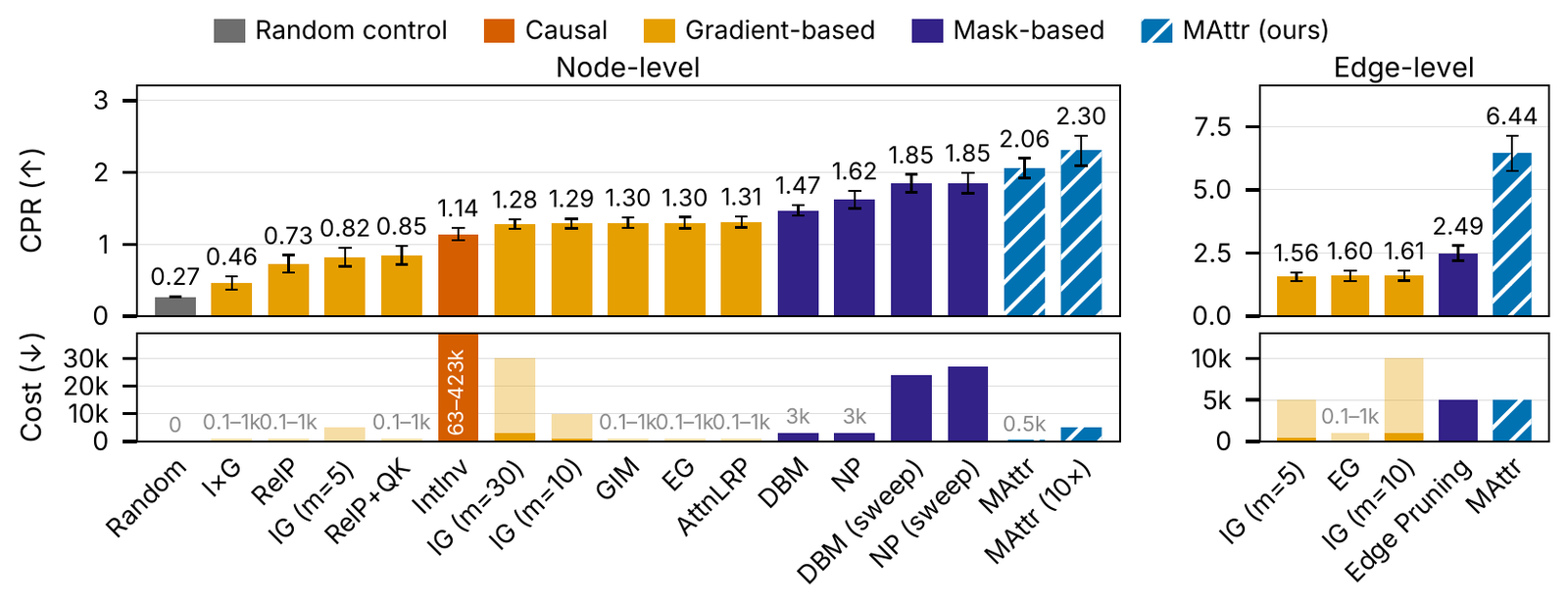
The "2.9×" is the edge-level entry on the official board, and the metric is CPR. The submission "MAttr (edge, 5k steps)" averages 5.6 across the 12 cells; the runner-up, an entry named "EAP + equiv linear maps of LLMs MLPs + G", averages 1.95 (measured, and the paper reports the same pair). 5.6 over 1.95 is 2.87 (reasoned). On the public split in Figure 2, edge-level MAttr scores 6.44 against 2.49 for Edge Pruning, about 2.6× (reasoned). The node-level margin is much smaller: 2.06 against 1.85 for the best sweep, about 11% (reasoned), or 2.30 with 10× the steps. A node-level MAttr submission was still pending on the board when I read it.
The per-cell picture, from the board (measured), with the best other entry in each cell whatever its coverage:
| Cell | MAttr CPR | best other CPR | MAttr CMD | best other CMD |
|---|---|---|---|---|
| IOI · GPT-2 small | 8.14 | 2.58 | 0.12 | 0.01 |
| IOI · Qwen2.5-0.5B | 3.73 | 1.88 | 0.09 | 0.01 |
| IOI · Gemma-2-2B | 4.36 | 3.33 | 0.27 | 0.03 |
| IOI · Llama-3.1-8B | 6.11 | 2.39 | 0.07 | 0.01 |
| MCQA · Qwen2.5-0.5B | 6.81 | 2.07 | 0.20 | 0.04 |
| MCQA · Gemma-2-2B | 3.78 | 2.59 | 0.25 | 0.04 |
| MCQA · Llama-3.1-8B | 6.05 | 1.84 | 0.54 | 0.12 |
| Arithmetic (+) · Llama-3.1-8B | 4.37 | 1.04 | 0.01 | 0.00 |
| Arithmetic (−) · Llama-3.1-8B | 4.74 | 1.07 | 0.02 | 0.00 |
| ARC-E · Gemma-2-2B | 4.06 | 2.39 | 0.22 | 0.03 |
| ARC-E · Llama-3.1-8B | 7.37 | 1.90 | 0.31 | 0.10 |
| ARC-C · Llama-3.1-8B | 7.65 | 2.04 | 0.25 | 0.11 |
| Average (11 full entries) | 5.6 | 1.95 | 0.19 | 0.06 |
MAttr leads CPR in all 12 cells. The paper states its per-cell lead ranges from 45.9% to 343.0%. The top of that range matches the board (arithmetic subtraction, 4.74 against 1.07), and 45.9% matches MCQA on Gemma-2 (3.78 against 2.59). But the smallest lead on the board today is IOI on Gemma-2, 4.36 against 3.33, about 31% (reasoned). I cannot tell from outside whether that is a later resubmission or a slip.
Paired Wilcoxon tests over the 12 cells give MAttr a 12/12 win against every node-level baseline except multi-sparsity Node Pruning, which it beats in 10/12, and 12/12 against every edge-level baseline run on all 12 cells (reported, Table 2, public test split). Across three seeds, the node-level average CPR has a standard deviation of 0.038 (reported, Table 3), although on ARC-C with Llama the headline seed scores 2.99 against a three-seed mean of 2.50.
Where it is not first
The table has a second pair of columns. CMD is MIB's other circuit metric, and on it the same submission averages 0.19 against 0.06 for the best entries (EAP-IG-inputs and a frozen-MLP EAP variant, both with counterfactual ablation): eighth of the 11 entries that cover every cell, and behind the best entry in every one of the 12 cells (measured). The paper reports CPR and its own Compactness metric; it does not report CMD for the headline runs.
The two metrics disagree because CPR is not bounded by 1. Faithfulness is a ratio of logit differences, so a circuit that leaves out the parts that work against the behaviour can score far above the full model. A CPR of 5.6 means that across the grid of circuit sizes, MAttr's circuits push the logit difference to several times what the full model produces. Its loss asks for exactly that. MIB's authors split faithfulness into two metrics for this reason: CPR "prioritizes methods that locate components with a positive effect on model performance"; CMD "components with any strong effect", including negative ones, and they suggest CMD when the aim is "to explain the full algorithm the model implements". A circuit that reproduces the model's behaviour and a circuit that maximises it are different objects.
The toy reproduces the split. Its suppressor N is a small version of the negative name-mover heads in the IOI circuit of GPT-2. With the headline loss, MAttr ranks N last, so its climbs to 1.18 by and stays there until N rejoins at ; its gap to 1 is 0.185, worse than IG's 0.179 (measured). Switch the loss to "match the model", which penalises (the repo implements this as the cmd loss), and N moves up to fifth: area falls from 1.042 to 0.935 and the gap halves to 0.091. The paper runs the same ablation on real tasks. Trained with the CMD-shaped loss, MAttr's average CPR drops from 1.67 to 0.96 while Compactness stays at 0.52 (reported, Table 8).
The authors do see CPR's flaws. They write that logit difference "is unbounded, so faithfulness can become far larger than 1", and they add Compactness: the area under interchange-intervention accuracy (does the circuit still prefer the base answer?) on a log-scaled size axis, which rewards small circuits that preserve the answer.
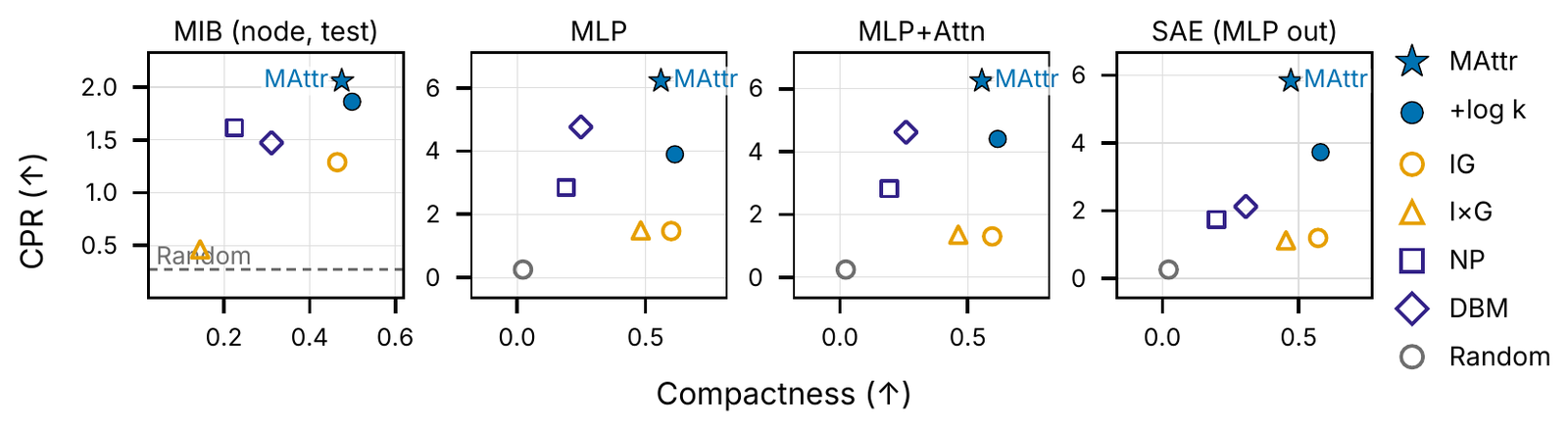
On Compactness the headline MAttr is not first either, once you go below the node level. On the MIB+ test set it scores 0.54 against IG's 0.51 at node level, but 0.56 against 0.60 on MLP neurons, 0.55 against 0.60 on MLP neurons plus heads, and 0.47 against 0.57 on SAE features (reported, Table 7). Sampling log-uniformly instead (the "+log k" variant) edges past IG on Compactness, at 0.61, 0.62 and 0.58, but its CPR falls to roughly two thirds of the headline's (reported scores, my ratio). The paper calls MAttr "close behind IG depending on the basis"; the budget distribution sets the trade-off.
One more limit: on IOI with GPT-2, every method the paper tests, MAttr included, ranks the backup name-mover head a11.h2 low (reported, Appendix H.1). The toy's backups are the only way a path survives; a real backup that activates only when its primary is ablated is harder to find.
Weights, not activations
The second half of the paper swaps the basis. Instead of activations of a base and a source input, it interpolates between two checkpoints of the same model: , with one score per -sized row of each weight matrix. The loss is a GRPO-style policy gradient on a judge's score, so the target does not need to be differentiable. Applied to base and instruct checkpoints of Llama with a refusal judge, it finds that restoring 1% of Llama-3.1-8B-Instruct's weights (2% for Llama-3.2-1B) to their base values removes most refusals (reported, Figure 5):
| Llama-3.1-8B | weights changed | StrongREJECT ↑ | GSM8K | IFEval | MMLU |
|---|---|---|---|---|---|
| Instruct | – | 2.6 | 81.0 | 74.7 | 69.1 |
| Abliteration | 27.6% | 68.6 | 81.5 | 76.2 | 68.6 |
| Expected gradients | 1.0% | 59.5 | 76.5 | 47.5 | 67.8 |
| MAttr | 1.0% | 84.0 | 79.5 | 71.7 | 69.5 |
At the same 1% budget, expected gradients breaks instruction following (IFEval 47.5) and MAttr mostly keeps it (71.7). On the 1B model MAttr's StrongREJECT score of 75.8 trails GRPO (86.4), GRPO with a KL penalty (89.3) and GRP-Oblit (78.7), which are allowed to change every weight. The paper frames this as an audit result: a released base checkpoint next to its safety-tuned sibling makes the refusal delta easy to localise. The single-direction ablation it compares against is the same mechanism covered in runtime abliteration.
Running it
The repo is one Python package (src/matryoshka_attribution/) plus experiment scripts, with a custom autograd function for the sigmoid top-k and a gradient-check test for it. At af82b2e it has no licence file for the code. The README's node-level recipe:
uv run python scripts/mib/eval_mib.py --model gpt2 --task ioi \
  --steps 500 --k-schedule uniform --masking topk --mode iso --lr 0.05 \
  --split validation --train-split train --include-input \
  --output results/mib_node_topk_uniform_lr05
--mode iso keeps the top clean and patches the rest, as MIB scores it; --mode cause does the reverse. Gemma-2 cells need a separate pinned TransformerLens 2.x environment. The weight-attribution code lives in a sibling repo, and the leaderboard circuits are on Hugging Face at aryaman/mattr-mib-circuits.
- branch
- HEAD
- tests
- 4 files
- source
- 2.2 MB
- commit date
- 2026-09-25
by size of tracked source at this commit, file counts in brackets; docs, data and vendored trees excluded
local clone, 2026-09-26 at af82b2e — branch, commit, commitDate, fileCount, hasTests, languages, shallow, testFileCount
shallow clone: counts describe the pinned tree, not the history
The take
MAttr turns circuit discovery into the objective the benchmark already uses (keep parts, patch the rest, see what survives), makes it differentiable with a soft top-, and trains it at every at once, so the answer is a ranking rather than one circuit. Its first step is IG; the training is what finds interactions, like the one backup that is enough. It is cheap next to patching and next to mask sweeps.
The headline needs its metric attached. MAttr is 2.9× the runner-up on MIB's edge-level CPR, a metric that rewards circuits for exceeding the full model, trained with a loss that asks for exactly that. On CMD, which asks a circuit to reproduce the model, the same submission is eighth of eleven, and on the paper's own Compactness it trails IG on the finer bases. Whether you want the parts that drive a behaviour or the parts that explain the model's computation is a choice the loss makes for you. For more on reading a model's internals, see the Jacobian lens, its cross-model follow-up and activation-probe monitors.
Built from arXiv 2609.25518, the matryoshka-attribution repo at af82b2e and the MIB leaderboard as read on 2026-09-26. Figures 1 to 3 are reproduced from the paper for commentary. The NestedMaskLab toy is my own; its numbers describe the toy, not a real model. Paper numbers are the authors' and I have not reproduced them.