2026-07-08 · 16 min · interpretability · transformers
Why read this
Notabletop 60%The Jacobian lens from the estimator up: why an averaged derivative beats the logit lens, where the tangent fails, and the two-call API to run it.
- Runs on a consumer GPU
- A lasting reference
- A new technique
InterpretabilityApache-2.0Research paper
How this was scored
- Is it new?
- 2 of 3: A real new idea, method or capability
- Can I trust it?
- 1 of 3: Spot-checks a few numbers
- Can I run it?
- 3 of 3: Open, permissive, runs on reader hardware with instructions
- Will I understand it?
- 2 of 3: Mechanism from first principles with figures
- Can I act on it?
- 2 of 3: A concrete recipe, numbers or comparison
- Will it last?
- 2 of 3: A reference for a year or more
- Does it affect many?
- 1 of 3: A specialist community
- Only here?
- 1 of 3: Some original analysis
Score 60 of 100, ranked 332 of 577 rated articles. Each question is answered 0–3 by hand, and a 3 is rare. How articles are scored
The Jacobian lens answers one question: given a model's internal state at some layer, what is that state disposed to make the model say? It is a small piece of code — Anthropic's jacobian-lens repo, Apache-2.0, "reference implementation, not maintained" — that fits on any open-weights decoder transformer and reads intermediate activations out as ranked vocabulary tokens. The whole method is one line:
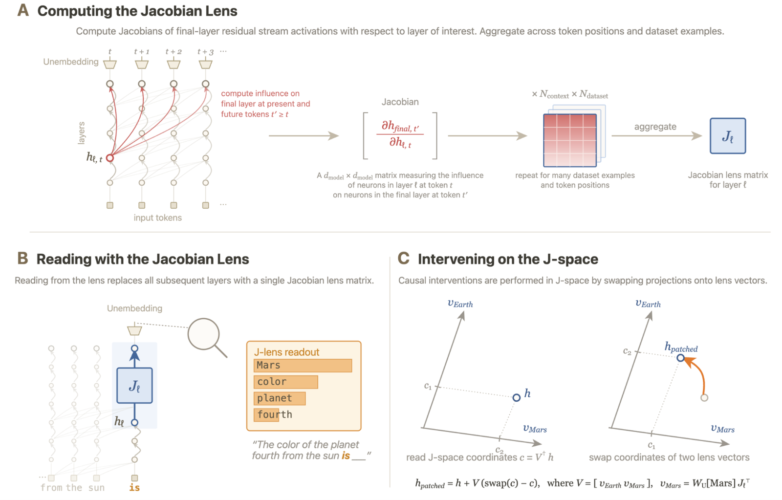
Two moves. transports a residual-stream vector at layer into the final-layer basis. Then the model's own unembedding decodes it into logits over the vocabulary. The transport matrix is a Jacobian — the derivative of the final-layer residual with respect to layer — averaged over a corpus. That is the entire idea, and it is worth being precise about, because the derivative is doing something the logit lens never could.
Why a derivative
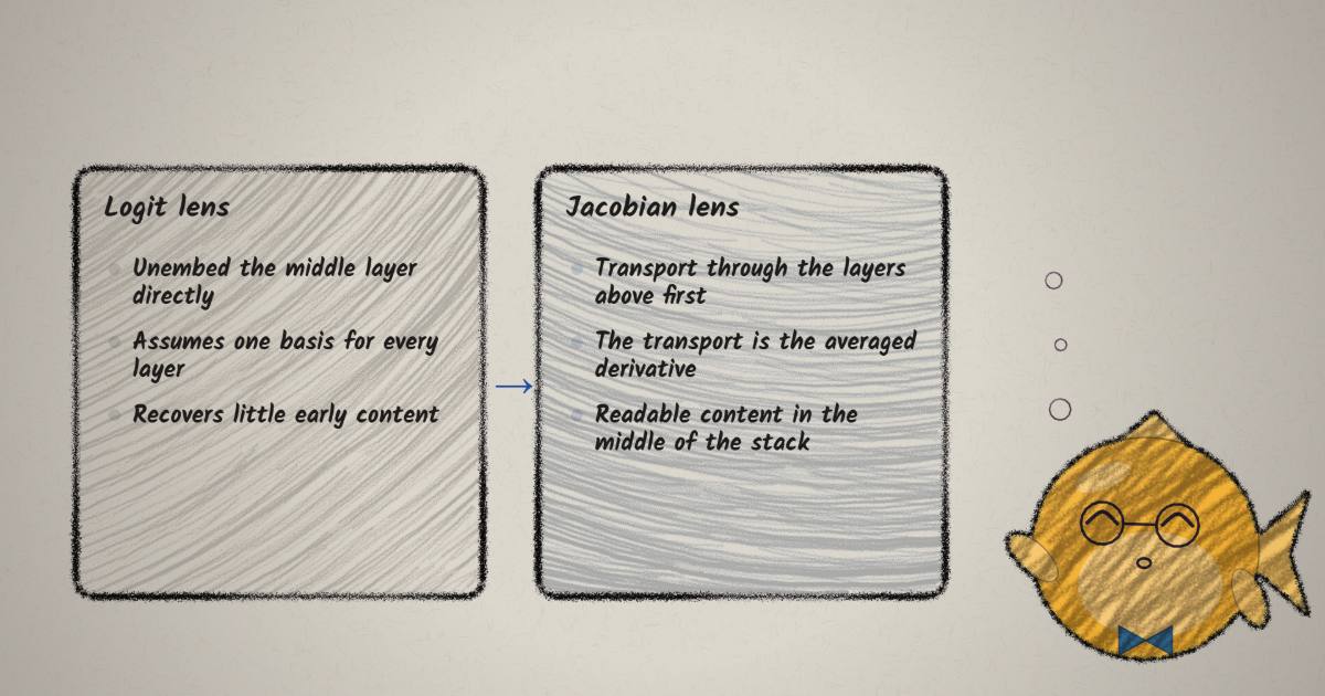
A residual stream is not written in the output vocabulary. The activation at some middle layer lives in a basis the model has been rotating and rewriting layer by layer; the unembedding only makes sense against the final layer. So you cannot just apply to a middle activation and expect a sensible token — the coordinates don't line up. That is the flaw in the logit lens, and the Jacobian lens is the fix: it first maps through the layers above it, then unembeds.
Mapping through the layers exactly would mean running the rest of the network — nonlinear, and no longer a "lens." The Jacobian is the linear stand-in. It is the best linear approximation to "run layers " around an operating point, and the repo takes that operating point to be the average over a text corpus. One matrix per layer, fit once, applied everywhere.
How the matrix is estimated
The estimator has one subtlety worth getting right. For a source position at layer , the influence on the final layer is not a single vector — it is spread over the current position and every future position (a decoder is causal, so can affect the output at ). The repo sums that influence over all target positions, then averages over source positions and over prompts. In the paper's own pseudocode:
# Compute J_ℓ for all layers ℓ.
# h_ℓ[t] : residual stream at layer ℓ, position t
# z[t]   : residual stream at the target layer L (final by default)
for each prompt p in corpus:
    run forward pass; cache h_ℓ[t] for all ℓ, t
    for i in 1..d_model:                    # one backward pass per output dim (batched)
        grad_z = e_i ⊗ 1_T                  # inject ∂/∂z_i = 1 at every position
        for each layer ℓ:
            G_ℓ = ∂(Σ_t z[t]) / ∂h_ℓ        # autodiff → shape [T, d_model]
            J_ℓ^(p)[i, :] = mean_t G_ℓ[t, :]  # mean over source positions
for each layer ℓ:
    J_ℓ = mean over prompts of J_ℓ^(p)      # aggregate the average Jacobian
# apply:
lens(h_ℓ) = softmax( W_U · norm( J_ℓ · h_ℓ ) )
Because is differentiated, a one-hot cotangent lands at every target position at once; causality makes vanish for , so what survives is exactly the sum over current-and-future targets. The paper's lenses use 1000 sequences of 128 tokens; the README notes quality "saturates quickly" and ~100 prompts is already usable. Cost is dominated by the model's own backward pass — one per output dimension, batched — which is why fitting is embarrassingly parallel across corpus slices (JacobianLens.merge()).
The rows of are the interesting object: the paper calls them the J-lens vectors, one per vocabulary token, each a direction in residual-stream space "associated with a single token."
A Jacobian is a tangent
Here is the mechanism I want to build intuition for, because it is also the method's main limitation. A Jacobian is a local linear map. Collapse the stack to one scalar activation coordinate and one token's logit, and the true function is a curve; the lens is its tangent line. Slide the probe below.
In local mode the tangent is re-taken at the probe, so it always touches — that is the textbook Jacobian, exact at the point and good nearby. But the real lens is corpus-average mode: one tangent, taken once at the corpus operating point, then used for every activation you feed it. Near that point the linear readout is faithful; far from it the error grows. This is the honest cost of turning "run the rest of the network" into a single matrix. The lens tells you what an activation is disposed to say to first order, on average; it is not a faithful simulation of the model from layer onward.
Then it is just a dot product
The second half, unembed(·), is the easy half. Unembedding is a matrix of one row per token; a logit is that row dotted with the transported vector. Softmax ranks them, and the lens readout is the top of the list — the token whose direction points most toward. Rotate the transported vector and watch the readout hand off between neighbouring concepts:
The superscript rank you see on a real slice page — nose³, smile¹⁰⁴ — is exactly a token's position in this sorted vocabulary. Rank, not just top-1, is what makes the lens useful: a concept can be climbing toward the top for several layers before it ever wins.
What it surfaces: the ASCII-face
The repo ships one example that makes the point in a single screenshot. Give the model an ASCII-art face and ask what it depicts. The ^ character is the nose. Select that position and the lens, at middle layers, reads out nose — a word that never appears in the prompt.
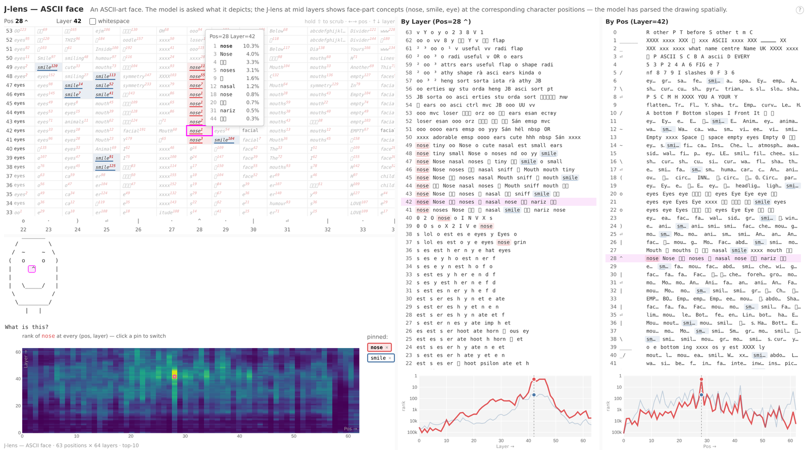
Reading the page: each cell is the lens top-1 word at that (position, layer); the bottom row is the model's actual output; the heatmap and line charts track a pinned concept's rank across the grid. The signal for "nose" is not at the output layer — it is a hotspot in the middle, then it fades as the model resolves what to actually say. That is the whole pitch: the lens shows intermediate content the output distribution has already moved past.
A lens is a choice of transport
Every "lens" is the same unembedding applied to a transported activation; they differ only in the transport .
| lens | transport | how it's obtained | early-layer behaviour |
|---|---|---|---|
| logit lens | identity | none | assumes one basis for all layers; recovers little early content |
| tuned lens | learned linear map | trained to match the output distribution (correlational) | tends to "skip ahead" to the output |
| Jacobian lens | fit by autodiff over a corpus | corrects for cross-layer basis change by construction |
The logit lens is the special case — it works only where the residual basis already matches the final layer, i.e. the last few layers, and the paper notes the J-lens "agrees closely" there and diverges earlier. The tuned lens also fits per-layer linear maps, but on a correlational objective (match the output), which the paper finds "skips ahead" and buries exactly the unverbalized intermediates you wanted to see. The Jacobian's objective is the derivative itself, which is why it recovers interpretable content at depths where the logit lens does not.
Does the readout mean anything causally
A readout is a correlation until you intervene on it. The paper's stronger claim is that the J-lens directions are causally privileged, and it tests this by swapping coordinates in the space those vectors span ("J-space", panel C above). The headline: split a concept vector into its J-space component and the orthogonal remainder, then swap along each.
The striking part is the budget: that J-space component carries a median of only 6–7% of the concept vector's variance, with ~93% in the orthogonal remainder — yet the small component drives the swap (59%) and the remainder barely moves it (5%). A few percent of the variance is doing almost all of the reportable work. Intervening at intermediate layers also propagates: swapping a concept mid-stack flips the model's top-1 output on a majority of trials, scaling with model size.
The companion result is ablation: project the top J-space contents out of the residual stream and multi-hop reasoning collapses toward zero, while shallow tasks — classification, comparison, factual recall — are essentially unaffected. Read together, the lens is not just labelling activations; the directions it finds carry content the model actually uses for the harder, chained computations.
What it can and cannot tell you
Honest boundaries, several of them the authors' own words:
- It is a linear approximation, and an average one. One Jacobian per layer, taken at the corpus mean, stands in for a nonlinear stack. The
LensTangentwidget is the whole caveat — faithful near the operating point, progressively wrong away from it. - Single tokens only. Each J-lens vector is tied to one vocabulary token. Concepts that span multiple tokens are not directly captured (the appendices discuss extensions). The lens sees "Mars," not "the fourth planet."
- Approximate and incomplete. The paper states plainly that the J-lens "only approximately and incompletely captures the model's underlying workspace structure," and that a "true workspace" may operate in layers the lens misses.
- A readout is not a mechanism. The lens says what an activation is disposed to output; it does not tell you the circuit that put it there. The causal swaps above are what upgrade a readout from suggestive to load-bearing — do the intervention before you trust the picture.
- It is a reference implementation. Not optimized, not maintained; fitting is dominated by the model's backward pass. Fine for research, not a production probe.
Running it
The API is two calls — fit (or download) a lens, then apply it at chosen positions:
import transformers, jlens

hf  = transformers.AutoModelForCausalLM.from_pretrained("org/model").cuda()
tok = transformers.AutoTokenizer.from_pretrained("org/model")
model = jlens.from_hf(hf, tok)

lens = jlens.JacobianLens.from_pretrained("org/lens-repo", filename="model/lens.pt")
lens_logits, model_logits, _ = lens.apply(
    model, "Fact: The currency used in the country shaped like a boot is",
    positions=[-2])
for layer, logits in sorted(lens_logits.items()):
    print(layer, [tok.decode([t]) for t in logits[0].topk(5).indices])
Fitting your own is jlens.fit(model, prompts=...); the walkthrough.ipynb notebook goes end to end and renders a slice page like the ASCII-face one.
The take
The Jacobian lens is a clean idea executed narrowly. Swap the logit lens's implicit identity transport for the real averaged derivative, and you get a readout that works in the middle of the network, where the interesting, not-yet-verbalized computation lives. The mechanism is a first-order Taylor term — a tangent — and the honest framing is exactly that: a good local, on-average picture of what a layer is disposed to say, not a faithful replay of the layers above it. What earns it more than "nice visualization" is the causal follow-through: a component holding ~6–7% of a concept's variance drives most of the reportable behavior, and ablating the J-space directions specifically breaks multi-hop reasoning while leaving shallow tasks intact. That is a real, testable claim about which internal directions the model uses to talk — reached with a derivative and an unembedding, and not much else.
Update, 13 October: J++ filters the Jacobians before averaging them
Added 13 October 2026.
Kola Ayonrinde (Anthropic Fellows) and Jack Lindsey (Anthropic) posted the J++ Lens, announced in a thread by @kzSlider. It keeps everything above: one matrix per layer, then . What changes is which derivatives go into the average. The LensTangent widget's corpus-average mode is the right picture. The J-Lens gives every operating point in the corpus an equal vote on the tangent. J++ asks which operating points produce tangents worth voting with.
What Jacobian Filtering does
I read the post and the released code (safety-research/jpp_lens, Apache-2.0, commit 93f02cd). Per layer:
- Cluster. Run -means with on layer- activations, projected to 64 PCA dimensions after centring and unit-normalising. The clusters are fitted on 1,000 WikiText-103 sequences. No labels are used.
- Fit one Jacobian per cluster. Average only over source positions whose activation lands in cluster . The backward pass uses LRP rules, as in the R-Lens.
- Mix the experts. Combine them with one learned weight each:
The weights are where the labels come in. A readout pair is an (item, intermediate) pair, for example the prompt about the web-spinning animal paired with "spider". Its margin is the best logit among the target's tokens minus the 10th-largest logit. A positive margin means a hit at recall@10. The code (rank_objective.py, fitter.py) maximises a sigmoid surrogate of the macro-averaged hit rate:
where is the spread of that item's logits. The search runs 200 Adam steps from three starts, and it keeps whichever iterate scores best on the exact metric. Weights may be negative. The post's "filtering" is this: bad clusters get weight near zero or below it. Nothing is thresholded.
The labels come from a 20% split of the same five tasks that the lens is scored on (DEFAULT_FIT_FRACTION = 0.2, stratified by task, measured in the code). The task files hold 93–107 items each (measured), so about 20 items per task set the weights (reasoned). The other 80% are held out. So the split is honest, but the dev set and test set come from the same distribution.
What "55% more faithful" means
Here "faithful" means recall@10: an item is a hit if its intermediate appears in the top 10 readouts at any of seven evenly spaced layers. That score is macro-averaged over five tasks: multihop, multilingual, typo, association and poetry. On Qwen3.6-27B, J++ scores 55.2%, the J-Lens 35.7% and the R-Lens 37.7% (reported). The post's TL;DR says "55% success", and the thread says "55% more faithful". The thread's reading works only by coincidence: 55.2 / 35.7 is a +54.6% relative gain (reasoned). Across six models, the median relative gain over the J-Lens is +63.5% (reported):
| model | J-Lens | R-Lens | J++ |
|---|---|---|---|
| Qwen3.5-9B | 34.2 | 37.5 | 55.0 |
| Qwen3.6-27B | 35.7 | 37.7 | 55.2 |
| Gemma 4 31B | 34.9 | 46.4 | 58.0 |
| Olmo 3 32B | 32.6 | 36.2 | 50.0 |
| Qwen3.5-122B-A10B | 24.4 | 23.2 | 48.4 |
| DeepSeek-V4-Flash (284B) | 30.5 | 47.4 | 61.4 |
Recall@10, %, reported (post, Table 1).
The earlier-layer claim is shown in figures more than tables. Figure 1's heart example surfaces the intermediate at layer 24, against layer 40 for the J-Lens. In the suppression case study, an instructed concept is visible by layer 24 with J++ and only from layer 40 with the J-Lens (reported, out of 64 blocks). The per-layer recall curve (Figure 2b) gives no table.
Why it might work, and what the evidence supports
The mechanism is the tangent caveat from above. Some regions of activation space have a poor linear approximation, and their Jacobians are noise that averaging cannot cancel because the noise is biased. The evidence that filtering does the work is the ablation table (Qwen3.6-27B, reported). Dropping Jacobian Filtering costs 11.7 points, LRP costs 6.6 and Readout Filtering costs 2.9. Routing each activation to its own cluster's expert scores 44.1, worse than the mix. So the gain comes from re-weighting, not from a piecewise map. The best single expert per layer reaches 50.2. At layers 8 and 16, 10 of 16 experts score below 2%.
Two caveats. First, is still one linear map, so the tangent caveat is reduced, not removed: one tangent, taken from better operating points. Second, the weights are fitted on the eval metric itself. With 8 numbers per layer that is little capacity to overfit. A leave-one-task-out fit, where no dev item comes from the scored task, still reaches 54.4 (−0.8, reported). Still, the lens is no longer unsupervised, and recall@10 is the one number it was tuned toward. The better evidence is the metric J++ was not tuned on. In the intermediate-swap causal eval its vectors flip the answer in 59.7% of trials, against 49.3% for the J-Lens (reported). With 67 trials, that difference is about 7 trials (reasoned). It points the right way, but on a small sample. None of this has been run on Anthropic's own models, and I have reproduced none of it.
Neuronpedia hosts an interactive J++ demo on Qwen3.6-27B, and the fitted lenses are on Hugging Face at koayon/jpp-lenses. At inference J++ is a drop-in for the J-Lens: the matrix has the same shape and costs the same.
Built on the jacobian-lens reference implementation (Anthropic, Apache-2.0) and the paper Verbalizable Representations Form a Global Workspace in Language Models. Figures reproduced from the paper (Figure 4) and the repo (assets/slice_vis.png) for commentary. The LensTangent and UnembedReadout widgets are my own illustrations of the mechanism, not measured traces; all quantitative results are paper-reported on Anthropic's own models and I have not independently reproduced them.