Matryoshka LM Suites: stop training the small models twice

2026-08-23 · 10 min · pretraining · speculative-decoding · distillation · efficiency · explainer

Nearly every open model release is a suite: 1B, 8B, 30B, 70B, trained separately on similar data, with the small ones often distilled from the big one afterwards. Nobody questions this, because each model has to exist independently at serving time and the obvious way to make a model exist is to train it.

Matryoshka Language Model Suites points out that a {1B, 8B, 30B, 70B} suite is 109B trained parameters, and that if you nest them properly it is 70B — one architecture, four detachable exits, and every smaller model distilled from the largest as a free by-product of the same forward pass.


Paper	arXiv:2608.09703 · Nathan Godey, Yoav Artzi (Cornell) · 10 Aug 2026 · CC BY-SA 4.0
Checkpoints	nthngdy/matryoshka-3B, with a `transformers`-compatible implementation
Suite	500M / 1.5B / 3B, nested into 3.2B trained parameters against Vanilla's 5.2B (−38%)
Compute	36% less than three independent runs; the token-matched baseline burns 57% more
Quality	within 0.5 points average accuracy at every size; better OOD perplexity at 1.5B and 3B
Spec. decoding	500M draft / 3B verifier: 2,650 tok/s vs 2,100 (26%), where the independent pair loses to plain decoding
Training	35B tokens of FineWeb-Edu · 52 GPU-days on B200 for both suites combined

nthngdy/matryoshka-3Bhugging face · snapshot 2026-09-08

parameters: 3.36B
repo size: 265.50 GB
architecture: MatriochkaForCausalLM
license: apache-2.0
downloads: 399
likes: 4
files: 14

parameters by dtype

F32 3.36B

The accounting

θ₁ ⊂ θ₂ ⊂ … ⊂ θ_M — every exit is a prefix of the next−39% parameters trained

3 independent runs5.20B trained

1.51B

3.19B

one nested run3.19B trained

+1.01B

+1.68B

exit 1B params

exit 2B params

exit 3B params

independent suite

5.20B

3 runs, 3 data passes

nested suite

3.19B

one run, distillation included

what the old way costs

+63%

to get the same set of exits

The saving is entirely a function of the shape of the suite, and it grows with how many mid-sized models you ship. Two sizes buys you little. The paper’s {1B, 8B, 30B, 70B} example turns 109B trained parameters into 70B; a five-size Llama-shaped ladder does better still, because everything below the top is being paid for twice under the usual arrangement.

Training compute tracks the same ratio, since both suites see the same tokens and forward cost scales with activated parameters. The measured figure is 36% rather than 38% — each exit still runs its own LM head. Read the other way round, which is how the results table does it: the token-matched baseline burns 57% more compute to reach the same three checkpoints, and gets no distillation for it.

The saving is not subtle and it is not a scaling-law argument. If the parameters of the small model are literally a subset of the parameters of the large one, then training the large one trains the small one, and the second run was redundant.

The catch — which is why nobody does this — is that "literally a subset" is a strong constraint. Early-exit architectures satisfy it, but they force every exit to share a hidden dimension, so a 500M exit and a 3B exit have to be the same width and differ only in depth. That is a bad shape for both of them.

The nesting

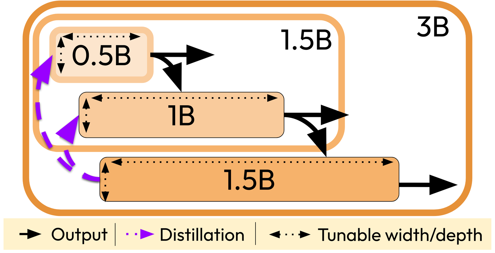
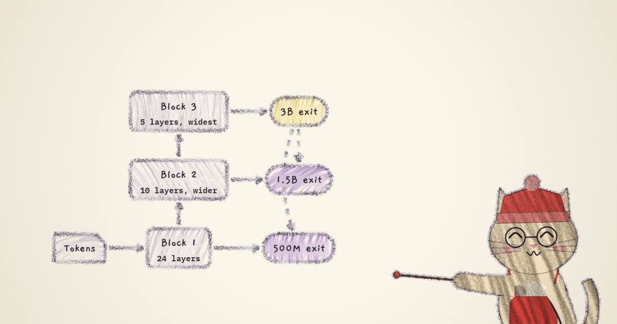
A diagram of three nested rounded rectangles labelled 3B, 1.5B and 500M from outside in. Inside, three horizontal blocks of increasing width labelled 0.5B, 1B and 1.5B are stacked, each with a black output arrow leaving to the right and a dotted double-headed arrow marking tunable width and depth. Purple dashed distillation arrows run from the largest block back to the two smaller ones. A legend identifies output arrows, distillation arrows, and tunable width and depth. — Sub-models nested into one architecture. Each block adds width and depth; each exit has its own LM head and can be detached and served as an ordinary checkpoint. (Godey & Artzi, Figure 1a.)

The paper's move is to let each sub-model have its own width and depth, and to solve the resulting dimension mismatch with a junction that adds no parameters.

When sub-model m hands its output to sub-model m+1, the output lives in D_m dimensions and the next block wants D_{m+1}. The naive fix is to concatenate a fresh embedding covering the new channels. That fails for a reason worth remembering: Transformer outputs have much larger norms than input embeddings, so concatenating them creates a magnitude mismatch that destabilizes training in the low-index channels. So the output gets rescaled first:

\tilde{o}^{m} = o^{m} \cdot \frac{\lVert e^{m+1} \rVert_2}{\lVert o^{m} \rVert_2}, \qquad o^{m+1} = T^{m+1}\!\left(\operatorname{concat}(e^{m+1}, \tilde{o}^{m})\right)

õ^m = o^m · ‖e^m+1‖ / ‖o^m‖ · then concat — no new parametersmagnitudes matched

õ^m carries information up from the sub-model below; e^m+1 is freshly initialized, exactly as a standalone model’s input embedding would be. Bar height above each band is its magnitude.

Both halves arrive at the next block at the same scale, so the low-index channels train like the rest.

Each sub-model also has its own LM head W_m and its own cross-entropy loss, so every exit detaches as a standalone checkpoint with its own depth and KV-cache footprint.

mismatch (illustrative)6×

what each half is worth — 200M proxy suite, average validation perplexity, lower is better

Vanilla suite (independent baseline)

20.05

three separately trained models — the target to land on

fresh embeddings + norm + distillation

20.07

the full recipe, within 0.02 PPL of the baseline

fresh embeddings + norm, no distillation

20.22

+0.15 — felt most by the smaller sub-models

fresh embeddings + distillation, no norm match

20.27

+0.20 — the magnitude mismatch, unmanaged

zero padding instead of fresh embeddings

20.61

+0.54 — off on every sub-model size

Turn the rescaling off and the picture shows the actual failure: the first D_m channels arrive carrying Transformer output magnitudes while the new ones arrive at embedding scale, and the next block has to learn across a cliff. The fix is one division and it adds no parameters — rescale the output so its norm matches the embedding’s, then concatenate.

The ablation prices both halves honestly. Zero padding instead of a fresh embedding is the worse mistake at +0.54 average perplexity; dropping the norm match costs +0.20. The full recipe lands within 0.02 of the independently-trained baseline — which is the number the whole nesting argument rests on, because near-parity at every exit is what makes the 38% parameter saving a saving rather than a trade.

39 layers, three exits, one run3.20B parameters trained

One architecture, 39 layers total, three exits. Each block is shorter and wider than the one below it — the depth triplet (24, 10, 5) was chosen from a sweep of every feasible split of 39 layers, to land on the Vanilla 3B's KV cache and per-token FLOPs simultaneously.

Flip between the two and watch the bars change direction. The Vanilla suite gets wider and deeper with size, as models normally do. The Matryoshka suite gets much wider and much shallower, because its blocks are increments rather than models: the 3B exit is five layers of width 4352 sitting on top of everything below it.

That shape is deliberate and it is the part most likely to be misread as arbitrary. The authors sweep every feasible way to split 39 layers into three blocks and pick (24, 10, 5) because it lands on the Vanilla 3B’s KV cache and its per-token FLOPs at the same time — 266 KB and 5.54 GFLOPs per token. Shallower budgets undershoot the memory footprint, deeper ones inflate the KV cache. The comparison is only fair because the shape was chosen to make it fair, which is a nicer piece of experimental design than it first looks.

Distillation for free

The second benefit is the one I would have led with. In a conventional suite, distilling the largest model into the smaller ones means either storing teacher logits offline or running the teacher alongside the student — significant compute or significant storage, either way.

In a nested suite, every forward pass through the largest sub-model already produced the logits of every smaller one. So the distillation term is:

\mathcal{L}^{M \to m}_{d} = -\sum_{v=1}^{V} \texttt{stop\_grad}\big(\sigma(l^{M})_v\big) \log \sigma(l^{m})_v

combined with each sub-model's own cross-entropy as (1 − α_d)·L_ce + α_d·L_d, summed over sub-models. The teacher costs nothing because it was already computed. The authors note that α_d wants to be lower than in offline setups — they use 0.3 — which is a small, believable detail of the kind that only shows up when you actually run the sweep.

Does it cost quality?

Essentially no, and this is where the paper is careful in a way that matters.

Comparing a Matryoshka suite to independent baselines is easy to rig, because you get to choose the shapes. So the authors fix the exit sizes, fix the head dimensions, sweep every feasible way to split 39 layers into three blocks, and pick the one that matches the Vanilla 3B on KV cache per token and per-token FLOPs simultaneously — 266.0 KB and 5.54 GFLOPs. They also give the 500M sub-model the identical width and depth in both suites, so at least one point is a strictly controlled comparison.

With that setup: near-parity on the seven-benchmark average at every size, within 0.5 points of the token-matched baseline that spent 57% more compute. Against the compute-matched baseline, Matryoshka wins at every size by +0.4 to +1.9 points. And on out-of-distribution byte perplexity it beats the token-matched baseline at 1.5B and 3B (2.121 vs 2.139; 2.067 vs 2.097), tying at 500M.

The speculative decoding result is the real payoff

Standard speculative decoding wants a draft one to two orders of magnitude smaller than the verifier: 60M for an 11B target, 160M–1B for 7B–70B Llama. Larger drafts do not amortize, because drafting cost and KV footprint grow faster than the acceptance rate they buy.

A 500M draft against a 3B verifier is a 1:6 ratio — well inside the unfavourable regime. The paper confirms it: the independently trained 500M/3B pair barely beats plain autoregressive decoding, and under nucleus sampling it is slower than not speculating at all.

E[emitted] = (1 − a^γ+1) / (1 − a) · 500M draft, 3B verifier, A100+0.50 tokens per cycle at γ = 6

agreement rate72.0% → 77.7%

what nesting removesindependent suiteMatryoshka suite

draft KV cachea second cache, held alongside the verifier'snone — the shared layers' cache is the verifier's

verifier work per cycleall 3.19B parameters, every verificationonly the 2.70B of blocks above the draft

max batch in 80 GB64102

throughput at draft length 6, greedy2,100 tok/s2,650 tok/s

Both curves flatten, and that flattening is the whole reason drafts are usually tiny. Past a certain length the marginal drafted token is almost never reached, but you pay to generate it on every single cycle — so drafting cost grows linearly while the return saturates. At a 1:6 ratio the draft is expensive enough that the two lines cross, which is exactly what the paper measures: the independently trained 500M/3B pair barely beats plain autoregressive decoding, and loses to it under nucleus sampling.

Nesting attacks that from three directions at once, and only one of them is the curve above. Sharing the KV cache removes the draft’s memory footprint entirely, which is worth a 59% larger batch in the same 80 GB. Sharing the layers means verification runs 2.70B of new blocks instead of 3.19B of everything. And weight sharing plus free online distillation raise the agreement rate, which is the one term everyone already optimizes. The same configuration that was a losing bet becomes a 26% speedup.

Nesting changes three things at once, and only one of them is the acceptance rate:

The KV cache is shared. The verifier's first 24 layers are the draft's layers, so the cache computed during drafting is reused directly. There is no second cache. In 80 GB that is the difference between a max batch of 64 and 102 — and a larger batch makes drafting cheaper relative to verification, because it is the bandwidth-bound half.
The layers are shared. Only the blocks above the draft need to run at verification: 2.70B of new parameters, not 3.19B of everything.
Agreement is higher. Weight sharing plus free online distillation raise cross-model next-token agreement by 5.7 points on the (1.5B, 3B) pair, with correspondingly lower KL. Independently trained models have no constraint pushing them toward each other and develop different representations.

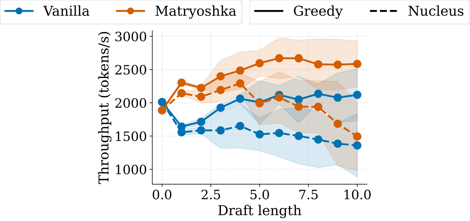
A line chart of speculative decoding throughput in tokens per second against draft length from zero to ten, with four series: Vanilla and Matryoshka, each under greedy and nucleus sampling, with shaded variance bands. At draft length zero all series meet near 1,900 to 2,000 tokens per second. The Matryoshka greedy curve rises to about 2,670 by draft length six and stays there; the Vanilla greedy curve reaches about 2,130. The Vanilla nucleus curve drops immediately below its own draft-length-zero value and declines throughout. — Draft length 0 is ordinary decoding. The independent pair's nucleus curve never returns to its own baseline — speculation costs it throughput at every draft length. (Godey & Artzi, Figure 5a.)

At draft length 6, Matryoshka reaches 2,650 tok/s greedy against Vanilla's 2,100 — a 26% speedup — and 20–40% over its own standard decoding, with the gain preserved under nucleus sampling.

There is an honest wrinkle in that figure that the paper does not dwell on and I think is worth naming: at draft length 0, the Matryoshka 3B is slightly slower than the Vanilla 3B (~1,890 vs ~2,010 tok/s). Thirty-nine layers is deeper than twenty-eight at the same parameter count, and depth costs latency. The speculative decoding win is large enough to swamp it, but if you are serving the 3B exit alone with no speculation, you are paying a few percent for the suite structure.

Against MatFormer

The obvious prior work is MatFormer, which also extracts nested sub-models from one run. The distinction is structural and shows up exactly where it matters at serving time: MatFormer nests along FFN width while sharing a single attention backbone, so every sub-model carries the same KV cache — 31.5 KB/token at 200M scale, whether you extracted the small one or the large one.

Matryoshka nests along depth, so the cache shrinks with the sub-model, down to 6.0 KB/token. At matched validation perplexity around 21, Matryoshka-100M matches MatFormer-M (139M) with roughly half the KV cache and fewer parameters; Matryoshka-200M reaches 17.92 against MatFormer-XL's 19.34.

The general point: a nested-model method is only useful if the small exit is genuinely smaller to serve, not merely smaller to describe. Parameter count is the easy half.

What I would want to see next

35B tokens is a proxy for something, and it isn't a real suite. The 3B suite trains on 35B tokens; production models at these sizes see 10–20 trillion. Everything about the nesting constraint — how much the shared trunk limits the largest model, whether the junction's norm rescaling stays stable, whether distillation from a heavily-trained teacher keeps helping the small exits — is a question about the regime this paper does not enter. The results are a strong existence proof, not a scaling claim, and the authors do not oversell them as one.

The depth budget was solved once, for one suite. L = 39 and the (24, 10, 5) split come from a ternary sweep against a specific baseline's footprint. That sweep costs a closed-form evaluation per candidate, so it is cheap — but it also means the recipe is "solve a small optimization problem per target suite" rather than a rule. A fitted heuristic for the depth triplet as a function of the exit sizes would make this deployable rather than reproducible.

The largest model has to give something up, and the paper cannot see it yet. The 3B exit is five layers of width 4352 sitting on 34 layers that were also optimized to be a good 500M and a good 1.5B model. At near-parity on 35B tokens that constraint is invisible. Whether it stays invisible when the top model is the one you actually care about is the question a lab would need answered before adopting this, and it is not answerable at this scale.

Every pair is a draft-verifier pair, and only one was measured. The paper notes that any (m, m') with m < m' forms a natural speculative pair, then evaluates 500M/3B. The 1.5B/3B pair is the one with the +5.7-point agreement gap — the largest in the paper — and 500M/1.5B is the cheap-draft configuration that conventional wisdom would actually pick. Both are one script away.

Why this one stuck with me

The compute saving is real but it is not what makes the paper good. What makes it good is that three separate things — suite training cost, distillation cost, and speculative decoding — turn out to be the same problem viewed from different angles, and one structural change addresses all three.

Suites exist because you want models at several sizes. Distillation exists because the small ones should learn from the big one. Speculative decoding exists because a small model that agrees with a big one can stand in for it. All three are statements about a small model being related to a large one, and the field's default answer to all three is "train them separately, then bolt on a mechanism that relates them afterwards".

Nesting relates them by construction, and then the mechanisms become free: the teacher's logits are already computed, the draft's KV cache is already the verifier's, the draft's layers are already the verifier's first layers. That is the kind of idea that reads as obvious after you have seen it, which is usually the sign it was not.