J-space in the open: a CKA map of workspace geometry across 38 models

2026-07-08 · 10 min · explainer · interpretability · transformers · llm

jspace-open is an interactive built by Elie Bakouch. It takes one idea from Anthropic's Verbalizable Representations Form a Global Workspace in Language Models — the Jacobian lens, which reads out the concepts a layer is disposed to say — and runs it across 38 open-weights models, 1,411 layers in total, from GPT-2 and Pythia up to Qwen3-32B and Llama-3.3-70B. Then it asks a single geometric question, cell by cell: do two layers arrange the vocabulary the same way? The map that falls out is oddly regular. Every model grows the same three-block layout — a sensory front, a workspace middle, a motor tail — and unrelated families put those blocks at nearly the same fraction of depth.

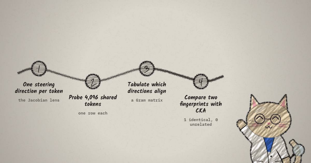
The J-lens vector: one steering direction per token, per layer

Start with what sits in each cell. The Jacobian lens asks: at layer $\ell$ , which vocabulary tokens is this activation pushing the model toward eventually saying? It answers with a linearized map from the layer's hidden state to the final residual stream, averaged over contexts:

J_\ell \;=\; \mathbb{E}_{t}\!\left[\frac{\partial h_{\text{final},\,t'}}{\partial h_{\ell,\,t}}\right]

Push a hidden state $h_\ell$ through it and read it out on the vocabulary:

\operatorname{lens}(h_\ell) \;=\; \operatorname{softmax}\!\big(W_U\,\operatorname{norm}(J_\ell\, h_\ell)\big)

where $W_U$ is the unembedding and $\operatorname{norm}$ is the final normalization. Turn that around and every token gets a direction. For token $t$ , its J-lens vector is the row of $(W_U\,\gamma)\,J_\ell$ — the direction in activation space that, added to $h_\ell$ , most raises the model's disposition to verbalize $t$ downstream ( $\gamma$ is the final-norm gain). It is a steering direction, indexed by (token, layer). The explorer probes each layer with the same 4,096 token strings shared by all 38 tokenizers, so the stack of directions at layer $\ell$ is a matrix

V_\ell \;=\; (W_U[\text{ids}]\,\gamma)\,J_\ell \;\in\; \mathbb{R}^{4096\times d}.

One row per probe token, $d$ the model width. Different models have different $d$ and different layer counts — which is exactly the problem CKA is built to sidestep.

What each cell measures: linear CKA on the token geometry

You cannot compare $V_i$ and $V_j$ coordinate-by-coordinate — different layers (and certainly different models) live in different bases and scales. So the explorer never compares coordinates. It compares the pairwise geometry of the 4,096 tokens. Center each layer's directions, then form its token-by-token Gram matrix:

\bar V_\ell = V_\ell - \operatorname{mean\ row}, \qquad K_\ell = \bar V_\ell\,\bar V_\ell^{\top} \in \mathbb{R}^{4096\times 4096}.

$K_\ell$ tabulates which tokens' steering directions align with which at layer $\ell$ — a pure relational fingerprint, independent of the basis. The cell value is the cosine between two such fingerprints — linear Centered Kernel Alignment:

\operatorname{CKA}(i,j) \;=\; \frac{\langle K_i, K_j\rangle_F}{\lVert K_i\rVert_F\,\lVert K_j\rVert_F}, \qquad 1 = \text{identical geometry},\; 0 = \text{unrelated}.

Because it only ever touches Gram matrices, CKA is invariant to rotation and isotropic scaling of each activation space. That invariance is the whole reason a 12-layer GPT-2 and a 64-layer Qwen — different widths, different depths, different training data — can share one axis at all.

Reading the big matrix

The headline view stacks all 38 models into one grid. Each block is a model against itself or against another; each cell is the CKA above.

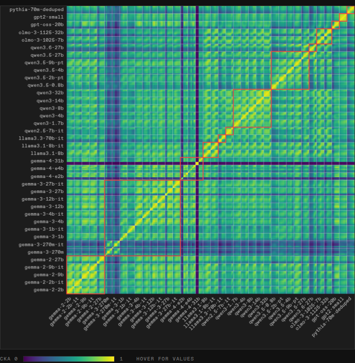
A large square heatmap in the viridis colormap. Bright yellow squares run down the diagonal — each is one model compared to itself, sub-divided by red outlines into family groups (gemma-2, gemma-3, qwen3, qwen3.5, etc.). Off-diagonal blocks compare two different models and show fainter teal 45-degree bands. Row and column labels list all 38 models from pythia-70m and gpt2-small up to qwen3-32b and llama3.3-70b-it. — The full 38-model J-lens CKA matrix — 1,411 layers × 1,411 layers. Bright diagonal blocks are within-model geometry; red outlines frame each sub-family; faint 45-degree bands in the cross blocks are two models organizing the vocabulary the same way at the same relative depth (Elie Bakouch, Fig 1).

Three things stand out. On each model's own diagonal, bright squares mark stretches of layers that hold one geometry — the paper's sensory / workspace / motor regions. In the cross blocks, a bright 45° band means two models line up at matched depth. And the red outlines separate within-family from across-family, so you can see that the band survives even when you leave a family — Llama next to OLMo, Gemma next to Qwen.

The interactive below rebuilds a single model's diagonal block so you can see the structure directly. Scrub the depth marker; switch the model. The values are a deterministic reconstruction of the pattern, not the measured matrix — but the geometry it encodes is the point:

within-model J-lens CKA · layer × layerillustrative

model

sensory workspace motor

relative depth (drag)

Each cell is the CKA between two layers’ token geometries: bright yellowon the diagonal (a layer is identical to itself), fading through teal to purple as two layers stop arranging the vocabulary the same way. The three outlined squares are the model’s sensory, workspace, and motor stretches — blocks of adjacent layers that share one geometry. Switch the model: the layer count changes from 32 to 64, but the block boundaries stay pinned at roughly the same relative depth (~47% and ~64%).

The layer count jumps from 32 to 64 as you switch models, yet the two block boundaries barely move in relative terms. That is the first surprise: the layout is a function of fractional depth, not layer index.

The reindex trick: same layout at the same relative depth

If the structure lives at relative depth, then to compare two models you have to put them on a common depth axis. The explorer's reindexed mode does exactly that — it resamples every block onto a shared 0–100% grid (bilinear), so matched relative depth becomes the 45° diagonal of every block. Raw mode keeps true layer counts; reindexed mode makes the alignment legible.

The widget below is the intuition without the heatmap. Six models, wildly different depths, each split into the three stages at the relative boundaries the explorer reports. Flip between raw and reindexed:

stage layout · reindexed 0–100%illustrative

layer axis

sensory workspace motor

On raw layers, a 12-layer GPT-2 and a 64-layer Qwen split into stages at wildly different absolute depths, and the boundaries scatter. Reindexevery model onto a common 0–100% axis and the same three regions snap onto the two guides — the explorer’s sensory / workspace / motorlayout, at nearly the same fraction of depth across unrelated families. That shared relative layout is what the CKA matrix picks up as a 45° band.

Raw, the boundaries scatter — a 12-layer model finishes its sensory phase in a handful of layers, a 64-layer model takes dozens. Reindexed, they snap onto the same two guides. That shared relative layout is precisely what shows up in the cross blocks as a diagonal band.

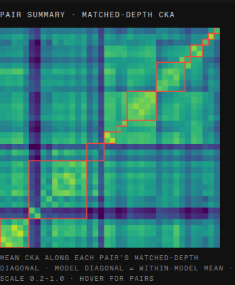
The explorer also summarizes each pair with a single number: the mean CKA along its matched-depth diagonal, $j(i) = \operatorname{round}\!\big(i\,\tfrac{L_B-1}{L_A-1}\big)$ , so "does layer 30% of A do the job of layer 30% of B?" collapses to one scalar per pair. Laid out as a model-by-model matrix, it is the same story at lower resolution:

A smaller square heatmap titled 'pair summary — matched-depth CKA'. Each cell is one model pair; the diagonal (a model versus itself) is bright yellow, off-diagonal cells are teal-green, and red outlines group families. A bright diagonal ridge runs corner to corner. — Pair summary: mean CKA along each pair's matched-depth diagonal, one cell per model pair (the model diagonal is the within-model mean), scaled 0.2–1.0 (Elie Bakouch, Fig 2).

How universal is it, really?

"Weirdly universal" is Elie's phrase, and the map earns it — but the honest version needs the numbers, because a bright block can hide a modest effect. For the full 38-model selection the explorer reports these cross-model means, averaged over all $\binom{38}{2} = 703$ pairs:

stat	value	what it is
off-diagonal block CKA	0.548	$\operatorname{BLK}=\tfrac{1}{L_AL_B}\sum_{i,j}C(a_i,b_j)$ — the depth-independent floor two models share
matched-depth CKA	0.588	$\operatorname{MD}=\tfrac{1}{L_A}\sum_i C(a_i,b_{j(i)})$ — the 45° diagonal only
depth-alignment gain	+0.040	$\operatorname{MD}-\operatorname{BLK}$ — similarity that is specifically at the right depth
block separation	+0.209	a model resembles itself more than it resembles others
depth order $\rho$	0.83	rank correlation of each layer's best-match depth (1.0 = order perfectly preserved)

Two of those numbers deserve a hard look. Most of the cross-model similarity is the lexical backbone: a floor of $0.548$ that every model shares simply because every model puts "dog" near "dogs." The part that is specifically about matched depth — the diagonal band over that floor — is only +0.040.

cross-model CKA (0–1) — provider tool, 38-model mean

block floor (lexical)

0.55

matched-depth

0.59

00.51

So the strong claim — "layer 30% of Llama and layer 30% of OLMo compute the same thing" — is not what the number supports. What the map actually shows is subtler and, I think, more interesting: the ordering is shared. Depth-order $\rho = 0.83$ says that as you walk down one model, the layer in another model that best matches you almost always walks down in step. Block separation $+0.209$ says the three-stage structure is a real, self-similar object, not an artifact of the lexical floor. The vocabulary geometry reorganizes in the same sequence, at the same relative pace, across families that never saw each other's data. That is the finding — a shared itinerary, more than a shared computation.

Where the pattern bends

The interesting parts of a "universal" map are the exceptions, and Elie flags a few. Base vs instruct checkpoints (Gemma-4 is the clearest) diverge most in the early, sensory layers — instruction tuning rewrites low-level parsing more than it touches the workspace middle, which stays put. Qwen3-32B reads as architecturally odd, looking like it skips or compresses an early phase — though that block is also the 80-prompt fit, so I would not over-read it. And on tokenizers: the shared 4,096 probe strings could in principle bias the comparison, but Elie checked with random token sampling and the pattern held, which is the right control to run.

The take

jspace-open is a good piece of interpretability tooling: it takes an Anthropic method that only Anthropic could run on Claude, points it at weights anyone can download, and lets you check the geometry yourself instead of taking it on faith. The honest read is a shared structure — three blocks, in order, at matched relative depth, with $\rho = 0.83$ and clean block separation — rather than a shared function, since the matched-depth lift over the lexical floor is only +0.040 and the block widths drift from the paper's Claude numbers. That is still a real result: open models from unrelated families grow the same coarse workspace itinerary. What the map does not do is re-establish that these directions are causally verbalizable — that remains a claim about Claude, and the mechanism behind the lens is its own story, covered in the Jacobian-lens explainer. Here, the contribution is the map: a way to see that the structure travels.

Primary source: jspace-open (Elie Bakouch, 2026), the J-lens CKA explorer. Built on Anthropic's Verbalizable Representations Form a Global Workspace and the neuronpedia/jacobian-lens lens weights. The two figures are screenshots of the explorer, reproduced for commentary; all stats are read directly from the tool's 38-model summary. The interactive diagrams are deterministic reconstructions of the pattern, not the measured CKA matrix.