2026-10-06 · 21 min · looped-transformers · recurrent-depth · mixture-of-experts · diffusion · image-generation · architecture · llm · explainer
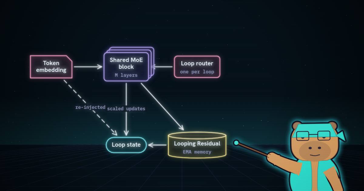
When this site covered SMELT, the main finding was a ceiling. Under matched FLOPs, parameters and KV cache, looping a MoE transformer's middle layers twice beat the unlooped baseline. Looping it three or four times did worse. A concurrent paper, "Loop the Loopies!", reached the same optimum of two under wall-clock matching. Nanbeige4.2-3B shipped with a loop count of 2. Three groups, one answer.
Two papers from the last week push past it:
- LOOM (arXiv 2610.01153, He, Li, Chang, Meng, Yin, Liu; code at hed-ucas/LOOM). It is a training recipe for looped MoE language models, and it reports stable training at 9-12 loops.
- Looped-DiT (arXiv 2609.40305, Chng, Chen et al., SenseTime and Tsinghua; code at OpenSenseNova/Looped-DiT). It loops the middle blocks of a text-to-image diffusion transformer inside each denoising step.
Looping is depth with shared weights
A standard transformer applies distinct blocks once each. A looped transformer applies the same blocks times:
Effective depth is , and the parameter count is still that of blocks. That is the whole appeal. The looped transformer architecture page covers the lineage: Universal Transformer, ALBERT, Huginn and Ouro.
The catch is that a model has three budgets, and looping moves only one of them:
- Parameters stay flat. That is the point of sharing weights.
- FLOPs per token grow about -fold, because every pass is a full forward pass through the shared blocks.
- KV cache also grows about -fold in an autoregressive model. Each pass runs attention on a different hidden state, so each pass writes its own keys and values.
A parameter-matched comparison is therefore a compute-mismatched one, which was this site's complaint about virtual logic depth. Huginn versus Ouro shows how many other design axes hide inside the word "looped". The first question for any looped result is which budget was held fixed.
Why two loops is where naive looping stalls
LOOM's diagnosis has two parts.
Variance growth (the curse of depth). In a pre-norm residual stream, . The norm keeps every update roughly the same size while the stream grows as updates pile up, so each new update moves the state relatively less and deep layers drift toward identity maps. Sun et al. called this "the curse of depth" (Shiwei Liu is an author on both papers).
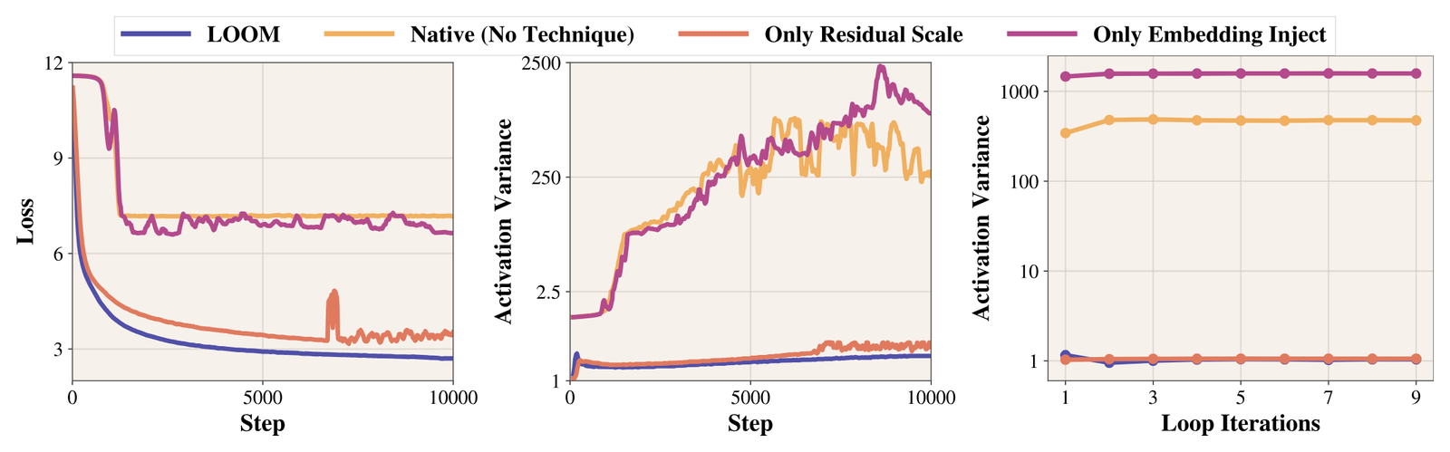
Looping makes it worse, because the updates are no longer independent. Ten different layers write roughly uncorrelated vectors, so their sum grows like . The same layer writing on its ninth visit tends to push in the same direction it pushed on visits one through eight, so the sum grows closer to linearly in . LOOM's Figure 3 shows this directly. On a 9-loop, ~350M model with no fixes, activation variance sits in the hundreds. With residual scaling it stays near 1 (reported).
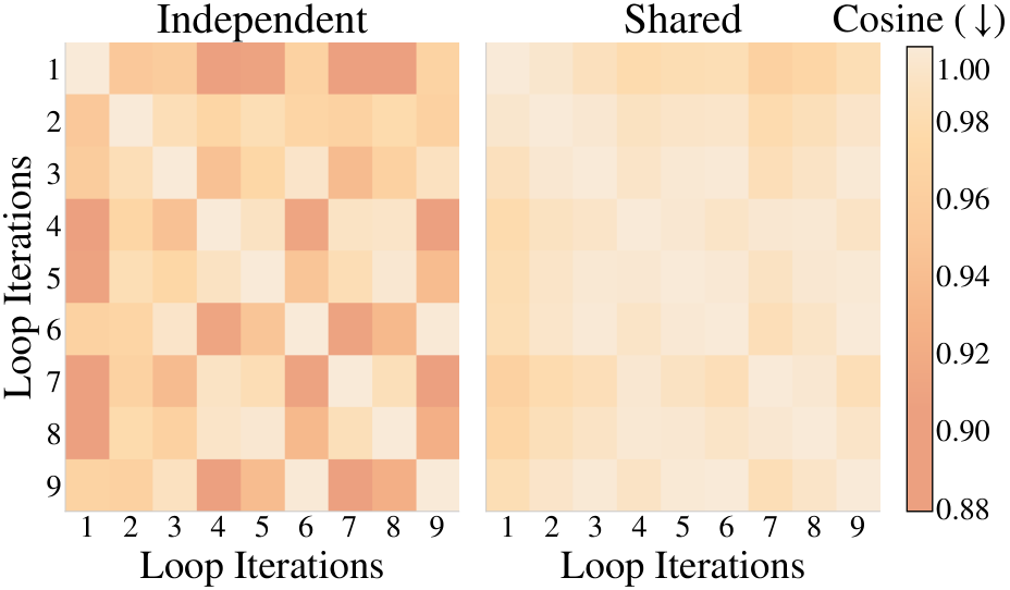
Expert-selection collapse. In a looped MoE, the router for layer is part of the shared block. The hidden state changes only a little between loops, so the router sends the token to nearly the same experts each time. The extra loop then re-runs a similar computation instead of a new one. LOOM's Figure 4 measures this as the cosine similarity of per-loop expert-load distributions. With one shared router, every pair of loops sits near the top of the scale, which runs from 0.88 to 1.00.
Without the variance fix, extra loops destabilize training. Without the diversity fix, they are stable but redundant. Either way the third loop does not earn its FLOPs.
The LOOM recipe
LOOM's stated principle is "each loop should contribute new computation while keeping the recurrent state stable." Three components keep the state stable and two make the loops differ:
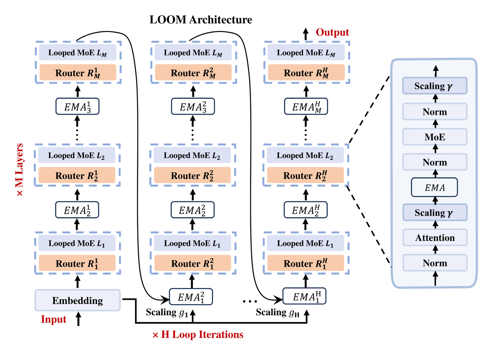
Residual scaling. Both the attention and MoE branch outputs are multiplied by
The two factors match the two kinds of accumulation. Across the layers of one loop, updates are roughly independent, so their sum grows like , and cancels that. Across the loops, the same layer's updates are correlated, so their sum grows like , and cancels that. Multiplied out, the total stays near times one update's scale, whatever the loop count (reasoned, from the paper's Eq. 1). The factor itself is from Wang et al.; LOOM applies it to MoE.
Embedding re-injection. At the start of each loop , the state is mixed back toward the input embedding:
For the 10-layer model, and (reasoned). The anchor is strongest early and fades, so late loops mostly refine their own state. Huginn re-injects the input too; the decay is new.
Loop-specific routers. Each loop gets its own router at every layer, while the expert weights stay shared. Router can send the same hidden state to different experts on loop 3 than on loop 7. In Figure 4 the shared-router matrix is nearly flat near the top of the scale. The per-loop matrix is visibly checkered, with loop pairs dropping to the bottom of its 0.88-1.00 colour range. The README's weave animation puts a number on it. Over 9 loops, one token of the 1.7B model touches 14 distinct experts at one layer, against 6 if every loop reused the same ones. Averaged over 16,384 held-out tokens it is 14.6, and two consecutive loops share about 3 of their 6 routed experts (reported, README).
The cost is small: at , , , five loops carry M router parameters in a 700M model (reasoned).
Looping Residual. This is the part that is new to LOOM. The direct attention residual is replaced by two exponential moving averages of the scaled attention outputs, each kept as an accumulator plus a scalar normalizer:
The global memory persists across all layers and loops. The local one resets at the start of each loop. The update becomes . With , the normalizer tends to 2, so the newest attention output carries about half the weight, the one before it a quarter, and so on (reasoned). Later loops see a summary of earlier loops' attention for one tensor and one scalar per memory. The paper writes both memories as fed by the raw attention output. The shipped scripts/train.sh sets arch.dual_axis_h_update_src=l, which feeds the global memory from the local summary instead (measured, models/dual_axis_carry.py line 823). Small, but the equation and the code that produced the numbers differ.
MoE output RMSNorm. The MoE branch output is RMS-normalized before scales it. The paper treats it as plumbing; the ablation says otherwise.
Segmented backprop, and the optimizer steps it adds
Backpropagating through 12 loops of an MoE stores 12 loops of activations. LOOM splits the loops into segments of at most . Each segment ends in an LM-head loss and a backward pass, and the hidden state and global memory are passed forward to the next segment with gradients detached. On the ~350M model with micro-batch 1, peak memory stays near 12.6 GiB from 3 to 12 loops, against 12.5 to 19.3 GiB without segmentation, and 12-loop training time drops from 26.1 to 12.6 hours (reported). Unsegmented 9-loop training also diverges: Table 6 lists a perplexity of 81.04 with an unrecoverable spike.
Algorithm 1 has one detail the prose does not spell out: line 10 reads "backward; optimizer step", and it runs inside the loop over . I checked the code. run_segmented_global_step in pretrain.py calls step_optimizers once per segment (measured). So a 9-loop model takes 3 optimizer updates per global batch and a 12-loop model takes 4, while the non-looped baseline takes 1. All of them see the same tokens and run the same learning-rate schedule, which is keyed to global steps. Each segment's loss also supervises loops 3, 6 and 9, not only the last. So segmentation is a memory trick and an optimizer change. The non-iso-FLOP results use it; the iso-FLOP results do not.
The numbers, with the arithmetic
M=10, 80 routed experts, 10B tokens. top-k shrinks as loops grow so f(H,k) stays near 84. Full backprop, no segmentation.
Where the fixed budget goes (reasoned from Eq. 5): attention costs 6 per pass, experts 3 per selected expert per pass. Looping at iso-FLOP moves compute out of experts and into attention.
Filled: LOOM validation perplexity, lower is better.
Iso-FLOP: best at 5 loops, and why that is a fair claim
The 700M experiment (Table 2) holds parameters fixed: , , 80 routed experts of width 512. It pays for extra loops by cutting top-. LOOM counts multiply-adds per token per layer in units of . Attention is : for grouped-query QKV, for causal SDPA and for the output projection. Each SwiGLU expert is :
I checked every row: , , , , , . They all match the table (reasoned). The SDPA term checks out too: at sequence length 1,024 , a causal token attends to keys on average, so and cost each. The uncounted router, about per loop, is under 1% of the budget (reasoned).
| Loops | Eff. depth | top-k | f(H,k) | Val. PPL | 7-task avg |
|---|---|---|---|---|---|
| 1 (baseline) | 10 | 26 | 84 | 18.36 | 38.84% |
| 2 | 20 | 12 | 84 | 17.37 | 39.00% |
| 3 | 30 | 8 | 90 | 16.91 | 39.34% |
| 4 | 40 | 5 | 84 | 16.58 | 39.53% |
| 5 | 50 | 4 | 90 | 16.54 | 39.53% |
| 6 | 60 | 3 | 90 | 16.57 | 39.50% |
Reported, LOOM Table 2. 700M parameters, 10B tokens, full backprop.
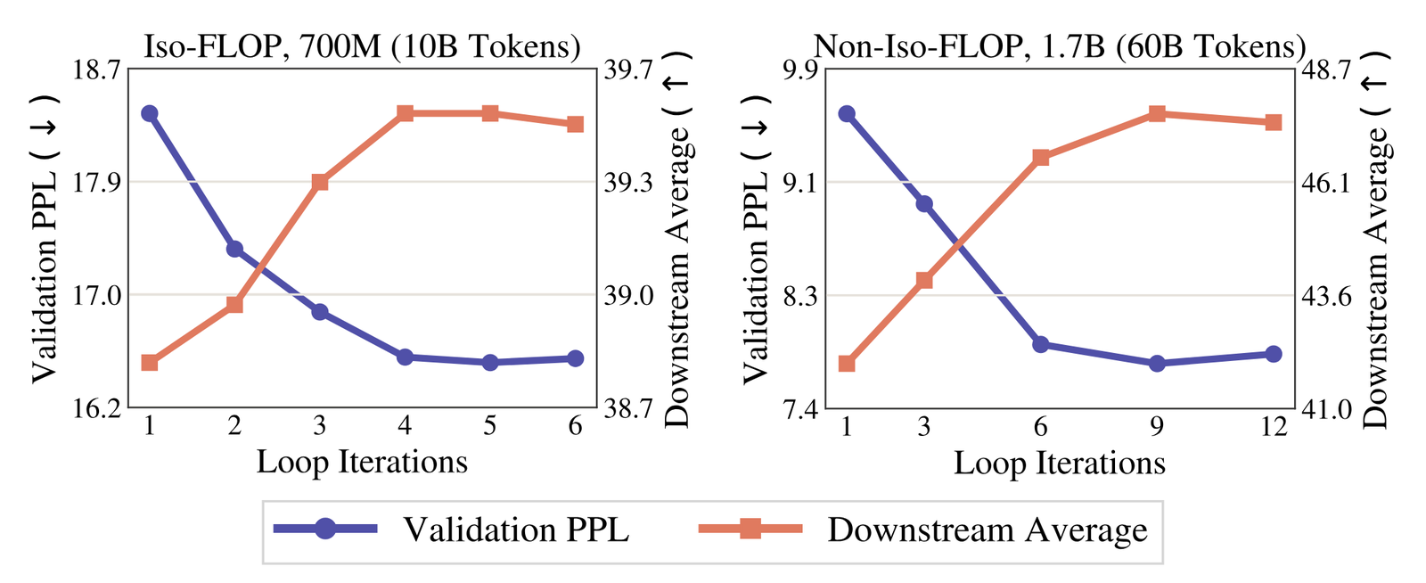
The headline row, 5 loops, spends , about 7% more FLOPs than the baseline (reasoned). The 4-loop row is exactly matched at 84 and reaches 16.58, within 0.04 of it. So "at matched FLOPs, looping beats the baseline, and the optimum is past two" survives the stricter reading: 18.36 → 16.58 at exactly equal cost (reported numbers, reasoned comparison). These runs use full backprop, so the segmentation confound does not apply. On the downstream average the gain is small: +0.69 points at 4 or 5 loops, and the paper reports no seed variance, so one run per setting cannot establish it. The perplexity gain is what this table really shows.
The widget shows what the paper does not: the compute is moved, not added. In the baseline, attention takes of the budget; at 5 loops it takes (reasoned). Iso-FLOP looping swaps a wide expert mixture (26 of 80 experts per token, a very dense MoE) for a narrow one run five times, with attention every time. Some of the win could come from spending more on attention, and the paper has no non-looped control with that split. The KV cache also grows fivefold, from 10 attention passes per token to 50. LOOM reports no inference memory or decode latency, so this is a training-compute claim. SMELT matched the cache; LOOM does not.
Iso-param: best at 9 loops, at about 9x the cost
At 1.7B parameters (0.63B active) and about 60B tokens, Table 4 reports:
| Loops | Eff. depth | Val. PPL | 7-task avg |
|---|---|---|---|
| 1 | 15 | 9.62 | 42.4% |
| 3 | 45 | 8.94 | 43.9% |
| 6 | 90 | 7.91 | 46.7% |
| 9 | 135 | 7.77 | 47.7% |
| 12 | 180 | 7.84 | 47.5% |
Reported, LOOM Table 4.
This is a real stability result: a 1.7B MoE trains through 135 effective layers and keeps improving up to 9 loops. On the ~350M backbone (Table 3), looping with no technique reaches a perplexity of 23.75 at 3 loops, already worse than the 20.07 baseline, and hits unrecoverable spikes with perplexity above 1,300 at 6, 9 and 12. LOOM's 9-loop run on that backbone reaches 14.80.
It is not a free lunch, and the paper's "unrolled scale of roughly 15B parameters (1.7B × 9)" invites a misreading. The 9-loop model costs roughly 9x the baseline's per-token compute in the looped blocks, to train and to serve, holds 9x the KV cache, and took 3 optimizer steps per batch to the baseline's 1 (reasoned; the optimizer count is measured from the code). The fair baseline is a model trained with 9x the compute, and the paper does not run one. SMELT's matched-compute frontier put the real saving from looping at 6.8-18.0% of training FLOPs. Read the 9.62 → 7.77 drop as "LOOM makes deep loops trainable", not as "loops are worth 9x".
Ablations
At ~350M and 9 loops, with every variant evaluated at step 5,000 (Table 5, reported):
| Variant | Val. PPL | Avg |
|---|---|---|
| LOOM | 18.62 | 39.8 |
| w/o residual scaling | 24.63 | 38.6 |
| w/o embedding re-injection | 26.05 | 39.2 |
| w/o MoE output RMSNorm | 26.50 | 39.0 |
| w/o Looping Residual | 19.25 | 39.3 |
| w/o per-loop routers (shared router) | 19.83 | 39.2 |
The stabilizers matter most: removing any one of them costs 6-8 perplexity points. The diversity components matter less: 0.63 points for the Looping Residual, 1.21 for the per-loop routers. Expert-selection collapse is real, but at step 5,000 it is the smaller problem. Whether that gap widens by the end of training is not reported.
Looped-DiT: the same idea inside a denoising step
A diffusion transformer already iterates over denoising steps. Looped-DiT adds a second loop inside each step, starting from MiniT2I, a minimal pixel-space MMDiT with 17 blocks (see the diffusion transformer architecture page). Those blocks are split into 6 pre-loop, 5 looped and 6 post-loop blocks, and the middle 5 run times. That gives block applications from 17 blocks of weights (reasoned, matches the paper's "effective depth 32").
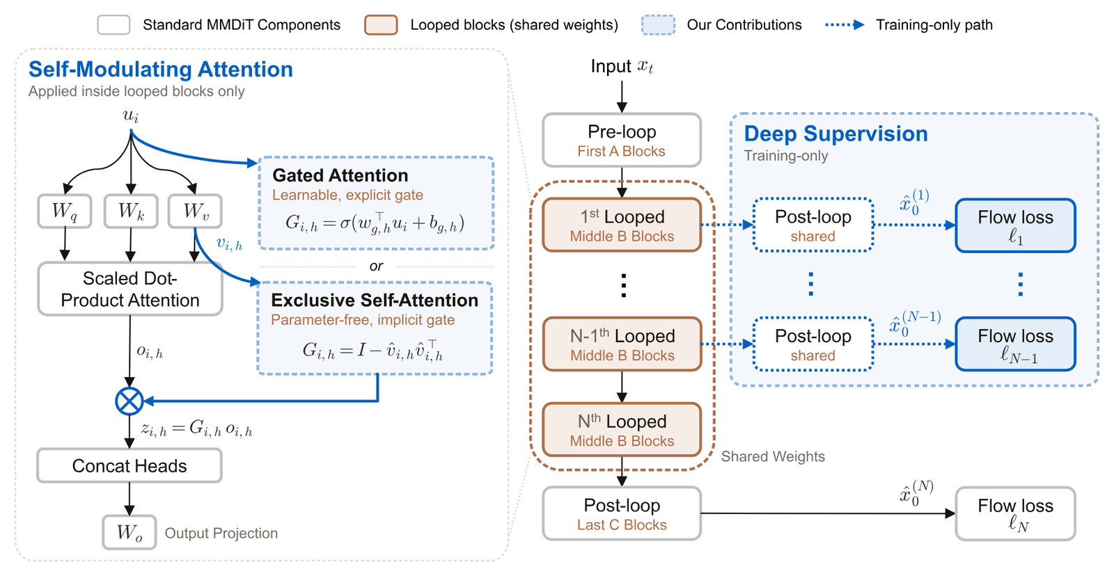
Naive looping has its own failure here, and the paper measures it. A ridge-regression probe that recovers each image token's 2D position from its hidden state drops from after loop 1 to after loop 8 (reported). Repeated attention updates overwrite where each patch is: the vision version of LOOM's drift. The two fixes:
- Deep Supervision. Every intermediate loop's hidden state is decoded through the same post-loop blocks, and its prediction is trained against the same clean image. Weights are , which the paper calls "Final + Mean". It costs training compute (1,246 GFLOPs per sample per step, against 809 for the looped model without it) but adds nothing at inference. Every loop becomes a valid exit.
- Self-Modulating Attention. Inside the looped blocks, each head's output is either scaled by a learned sigmoid gate or projected off the token's own value direction. The second option is Exclusive Self-Attention (XSA): . The paper's Eq. 6 describes XSA as dropping the term of the attention sum. The code (
exclusive_self_attentioninlooped_dit/model.py) projects the whole output, which also removes the part of every other token's value that lies along (measured). XSA beats the gate in the B/32 ablation, 58.5 to 56.6.
The ablation stacks up cleanly on B/32 (Table 4, four-benchmark average, reported): no loop 55.2, naive loop 56.2, plus Deep Supervision 57.5, plus XSA alone 58.5, both 59.1. XSA on a non-looped model does nothing (−0.1). On the looped model it adds +1.6 (Table 5). That fits the claim that it damps repeated updates, not attention in general.
Checking "6.5x larger" and "4.9x"
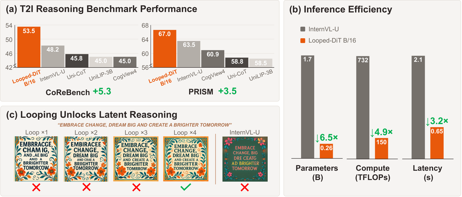
The abstract says a 260M looped model "can surpass a model 6.5× larger … while requiring 4.9× lower inference compute." Both ratios come from comparing against InternVL-U. In Figure 1(b) the parameter bars read 1.7 and 0.26 (billion), and . The compute bars read 732 and 150 TFLOPs per image, and . Latency is 2.1 s versus 0.65 s on one H100, (reasoned from the reported bars). The numbers are consistent. The X post that circulated the paper says "4.9x fewer parameters". That is wrong: 4.9x is the compute ratio, and the parameter ratio is 6.5x.
Two caveats. "Surpass" is on the six-benchmark average, 71.5 versus 69.0 (Table 1); Looped-DiT does not win GenEval (87.4, against 90.3 for UniLiP-3B). And the paper's training-data appendix describes the MiniT2I setup (CC12M, then BLIP3o-60K, DALL-E 3 and ShareGPT-4o-Image), while the shipped configs/b16_pretrain.yml also pretrains on FLUX-Reason-6M and configs/b16_finetune.yml mixes in Fine-T2I at weight 0.116, about half the samples (measured). The B/16 headline model saw more, and more reasoning-flavoured, data. I could not confirm what the MiniT2I-B/16 row (66.4) was trained on. The clean evidence is the B/32 work, where data is fixed.
Loops versus denoising steps
A diffusion model already has a knob for inference compute: more denoising steps. Figure 6 compares 4 loops at 25, 35 and 50 steps against 1 loop at 50, 70 and 100 steps, matched on per-image FLOPs.
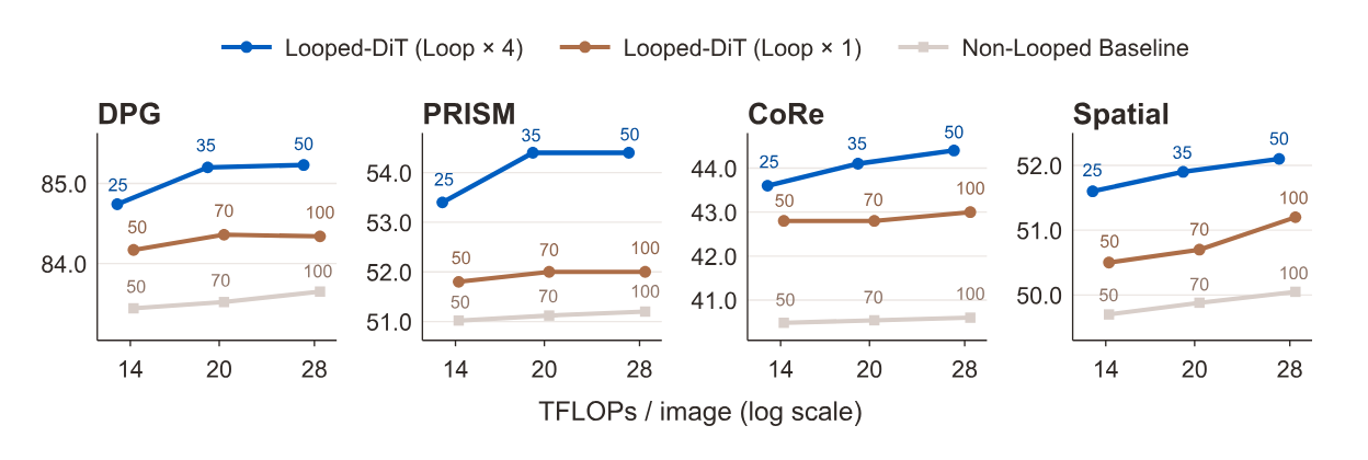
The FLOPs do match. Table 8 gives 146 GFLOPs per denoising forward pass with one loop and 267 with four, a ratio of 1.83, not 4, because the pre- and post-loop blocks run once either way. Then 25 steps × 267 = 6,675 GFLOPs and 50 steps × 146 = 7,300. If each step runs two passes for classifier-free guidance, these become about 13.4 and 14.6 TFLOPs, the "14" column of the plot (reasoned). The looped arm spends slightly less, and in every panel 4 loops at 25 steps beats 1 loop at 100 steps, which costs twice as much. My reading: past a few dozen Euler steps, more steps re-solve the same ODE more finely, while more loops give each step more depth to work out the layout, as in the sign that is misspelled at loops 1-3 and right at loop 4.
Diffusion also avoids LOOM's serving problem: a denoiser keeps no KV cache across steps, so looping costs FLOPs and latency, not cache memory (reasoned). Table 2 is honest about where the bill lands. Looped-DiT B/32 scores 59.1 against 58.1 for an untied 32-block model with the same Deep Supervision, but costs about 1.54× the training compute of the plain deeper and wider baselines, and the paper says so.
What carries across
The two papers solve the same problem in different domains, and their fixes rhyme:
| Failure | LOOM (MoE LM) | Looped-DiT (T2I diffusion) |
|---|---|---|
| State drifts or blows up | Residual scaling by plus MoE output norm | XSA or gate damping attention updates |
| Loop forgets its input | Decaying embedding re-injection | Probe shows positions eroding; XSA keeps highest |
| Loops repeat each other | Per-loop routers, Looping Residual | Not addressed: no experts to route |
| Only the last loop learns | Segment losses at loops 3, 6, 9 (a side effect) | Deep Supervision on every loop, by design |
Both papers show that loop count is a property of the training recipe, not of the architecture. "Two loops is optimal" was true of naive recipes; these move the optimum to 4-5 under near-matched FLOPs (LOOM) and to 4 trained loops with useful exits on either side (Looped-DiT). Neither shows that deep loops are cheap. LOOM's deepest wins are paid for in compute and cache; Looped-DiT's in training compute, at 0.26B scale.
The runs I'd want next: LOOM's iso-FLOP grid with the KV cache matched too; the 1.7B 9-loop row against a non-looped model given the same total compute and optimizer steps; and Looped-DiT at billions of parameters. Both codebases are public (Apache-2.0 and MIT), so all three are runnable.
- license
- Apache-2.0
- branch
- main
- tests
- none found
- source
- 572.2 kB
- commit date
- 2026-10-05
by size of tracked source at this commit, file counts in brackets; docs, data and vendored trees excluded
local clone, 2026-10-06 at a2ee5a7 — branch, commit, commitDate, fileCount, hasTests, languages, license, licenseFile, shallow
shallow clone: counts describe the pinned tree, not the history
- license
- MIT
- branch
- main
- tests
- 1 file
- source
- 132.7 kB
- commit date
- 2026-10-05
by size of tracked source at this commit, file counts in brackets; docs, data and vendored trees excluded
local clone, 2026-10-06 at 65a7705 — branch, commit, commitDate, fileCount, hasTests, languages, license, licenseFile, shallow, testFileCount
shallow clone: counts describe the pinned tree, not the history
For the routing basics see the mixture-of-experts architecture page, and for where expert routing time goes in practice, Halo's breakdown.