Lattice Deduction Transformers: reasoning by narrowing a lattice, not emitting tokens

md json mcp

2026-10-02 · 18 min · llm · looped-transformers · recurrent-depth · reasoning · neurosymbolic · formal-methods · small-models · explainer

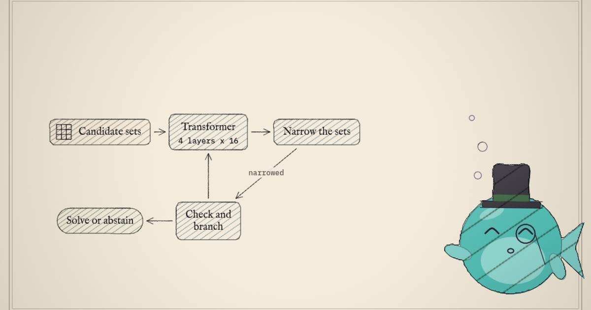
An 800K-parameter model solves Sudoku puzzles that Claude Opus 4.6, DeepSeek V4-Pro and GPT-5.4 cannot touch. Not "solves better" — the frontier LLMs score exactly 0% (reported), and the small model reports 100% (reported, with an asterisk I will get to). It trains in about fifteen minutes on a single GPU from a thousand example puzzles.

The interesting part is not the size. It is that the Lattice Deduction Transformer (LDT), from Liam Davis (Amherst), Leopold Haller and Alberto Alfarano (Axiom Math), and Mark Santolucito (Barnard) — arXiv 2605.08605 — does not reason the way a language model reasons. It never emits a token of chain-of-thought. Its working memory is not an opaque latent vector. It is a grid of candidate sets: for every cell, the set of digits still considered possible. The model's whole job, repeated pass after pass, is to cross candidates off that grid without ever crossing off the right one. That constraint — never remove a value the true solution needs — is called soundness, and it is what lets the system do something no LLM solver does: when it cannot finish, it says so instead of guessing wrong.

This piece walks the mechanism from first principles — the lattice, the looped transformer, the search loop — then holds the headline numbers against the primary sources, including a correction the authors themselves published and a follow-up paper arguing the whole thing is less clever than it looks.

Why Sudoku-Extreme breaks language models

Sudoku-Extreme is not newspaper Sudoku. The benchmark (introduced alongside HRM) filters the Tdoku generator down to puzzles that require search — instances where no sequence of human-style deductions finishes the grid, so any solver, symbolic or neural, has to guess a value, follow the consequences, and be ready to take the guess back. A symbolic solver does this with explicit backtracking. The question is what a neural network does.

An autoregressive LLM has no good answer. It reads the puzzle, emits digits left to right, and once a token is written it is in the context forever. There is no retract. The model can be told to "think step by step," but the thinking is more tokens in the same append-only stream; a wrong commitment early poisons everything after it, and the model has no typed notion of "this branch is dead, undo it." This is why a 1.6-trillion-parameter model (DeepSeek V4-Pro, reported) scores zero on a task a 0.0008-billion-parameter model saturates. The frontier LLM is playing the wrong game.

The family LDT belongs to has been building the right game for a while: looped and recurrent-depth transformers that reuse a small stack of weights many times instead of stacking many distinct layers. HRM uses a dual-loop recurrent architecture; the Tiny Recursive Model (TRM) shows a 2-layer network with recursion can beat it; Sotaku is a recurrent transformer specialised for Sudoku. This site has covered the lineage — what looping actually buys, what separates a good looped model from a bad one, and reasoning in hidden states rather than the token stream. LDT's contribution: make the thing the loop carries between passes not a hidden vector but an explicit, interpretable, sound object — a lattice.

The lattice, from the top

The word "lattice" here is the one from abstract interpretation, Cousot and Cousot's 1977 framework for sound approximate reasoning. The idea: replace exact computation over an expensive concrete domain $C$ with cheap computation over an abstract domain $A$ , in a way that guarantees any property you prove in $A$ holds in $C$ . You lose completeness — the abstraction may fail to prove something that is in fact true — but you never prove something false. For search problems, you buy completeness back with search.

For a 9×9 Sudoku, make it concrete. The concrete domain $C = \mathcal{P}(S)$ is the powerset of all fully-filled grids $S$ : an element is the set of complete grids still considered viable. Order it by inclusion — a smaller set is more informative — so $\top$ (top) is "every grid is possible, I know nothing" and $\bot$ (bottom) is the empty set, "no grid works, this is impossible."

Tracking literal sets of grids is hopeless. So abstract: for each cell, keep only the set of digits that appear there across the surviving grids, and throw away all the correlations between cells. That is the grid powerset lattice

A = \big(\{1,\dots,9\}^2 \to 2^{\{1,\dots,9\}}\big),

a map from each cell to a subset of the digits. Order it pointwise: $a' \sqsubseteq a$ when $a'(c) \subseteq a(c)$ for every cell $c$ . Here $\top$ gives every cell the full digit set, and $\bot$ is reached the moment any cell's candidate set goes empty. The two domains are tied together by an abstraction function $\alpha : C \to A$ (collect the digits appearing in each position) and a concretization $\gamma : A \to C$ (all grids whose every cell lands in the allowed set); they form a Galois connection, which is the formal condition that makes abstract proofs transfer to the concrete.

The most precise sound deduction step is then exactly

\mathit{ded}_p(a) = \alpha\big(\gamma(a) \cap \lVert p \rVert\big),

where $\lVert p \rVert$ is the set of valid solutions to puzzle $p$ : concretize, intersect with the real solutions, abstract back. In words — keep only the candidates that survive in at least one valid solution, and drop the rest. Classic Sudoku moves like naked singles and hidden singles are special cases. The point of soundness is that this operator only ever removes candidates, and it never removes a digit a true solution needs. The catch: computing $\mathit{ded}_p$ requires knowing $\lVert p \rVert$ , which is the whole problem. LDT's move is to train a transformer to approximate $\mathit{ded}_p$ from solution samples, without ever constructing $\lVert p \rVert$ explicitly.

Storing the lattice in a tensor

The lattice state becomes a multi-hot tensor: $|V|$ binary sigmoids per cell — $9 \times 9 \times 9 = 729$ sigmoids for a 9×9 board. Each sigmoid is the model's confidence that one candidate is still alive in that cell, and deduction means pushing sigmoids toward zero until every cell has a single survivor. A solved grid is one-hot per cell; the abstraction $\alpha$ over a set of solutions is a bit-level OR. Bottom gets a dual representation: implicitly, any cell whose candidate set is empty; and explicitly, a sigmoid on a dedicated [CLS] token trained to fire on any unsatisfiable state. That second channel matters later.

A diagram of the lattice-tensor encoding. On the left, a [CLS] token holding a bottom symbol, then rows labelled cell 1, cell 2, through cell n, each a strip of nine boxes numbered 1 to 9 with some boxes highlighted (alive candidates) and others greyed (eliminated). An arrow feeds all rows into a central Transformer block, which emits the same layout on the right, where cell 2 has collapsed to a single highlighted candidate. — The lattice as a tensor: one strip of nine candidate sigmoids per cell plus a [CLS] conflict channel, in and out of the transformer. In the output, a cell has collapsed to a single survivor — one deduction step (LDT, Figure 2).

The loop: four layers, sixteen times, re-reading the lattice

The network itself is small and plain. It is a recurrent transformer closely following Sotaku: a stack of 4 attention layers unrolled for 16 internal iterations, where the output of one iteration is the input of the next. The input lattice encoding is re-injected as a residual at every iteration — the same "keep showing the loop its input at every pass" move that the controlled ablations on looped models found to be one of the two changes that actually matter. Position is a learned 2D embedding (with 2D RoPE added inside attention for the larger maze grids). Every one of the 16 iterations emits its own candidate and conflict logits and is supervised; at inference only the final iteration is read out.

The LDT method diagram. On the left, a Hasse diagram of the powerset lattice of the set {1,2,3,4}, from the full set 1234 at the top down to the empty set at the bottom, with a red arrow marking a deduction step from node 234 down to node 3. On the right, a recurrent transformer: a lattice-encoding input box feeds a dashed block containing an Attention LayerNorm, a Multi-Head attention, a Forward LayerNorm, and a Feed layer, annotated as repeated 4 times and unrolled 16 times, with a Branch feedback path and the lattice-encoding re-injected, producing a lattice-encoding output. — LDT performs sound deduction on a lattice (left: a deduction step is a move down the order) using a recurrent transformer — four attention layers, unrolled sixteen times, with the lattice re-injected each pass and a branch step feeding search (LDT, Figure 1).

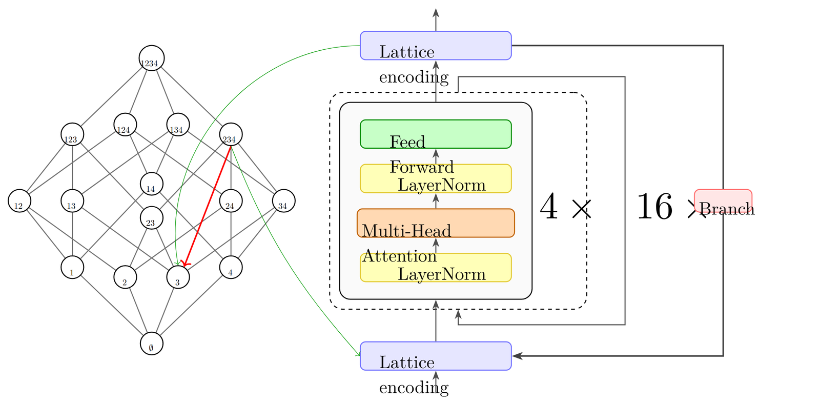
The structural difference from TRM and HRM is what the outer loop carries between search steps: not an opaque latent embedding but the lattice itself — a typed object you can read, whose moves are guaranteed sound. The transformer does the pattern-matching; the lattice does the bookkeeping. (The authors note the traces look a lot like a discrete-diffusion process — iteratively committing information about a partially-masked grid — recast as a fixed-point computation over an order.)

The search loop: deduce, branch, detect, backtrack

Approximating $\mathit{ded}_p$ is only half of it. Because the learned operator is sound but incomplete, deduction alone stalls on hard instances. So LDT wraps the transformer in a DPLL-style search — the same Solve procedure run at both training and inference, which is what keeps the training states in-distribution with what the model sees when it runs for real. One step, straight from the released code (experiments/sudoku/dpll.py):

Deduce (unit propagation). Run the transformer, read the per-candidate sigmoids, and eliminate every candidate whose probability falls below a threshold $\theta_{\text{elim}} \approx 0.1$ (measured — the threshold default in the code). This is deterministic and monotone: it only removes candidates.
Check. If every cell is a singleton, the grid is solved. If a cell is empty, or the [CLS] conflict head fires above its threshold, the state is $\bot$ — a conflict.
Branch (decision). Otherwise pick a cell with two or more live candidates uniformly at random, and pin it to a single digit sampled from a softmax over its alive candidates at temperature $\tau_{\text{decide}} = 1.5$ (measured — temp_decide in the code). This is the guess.
Backtrack. On conflict, reset the chain and try again. Termination is guaranteed because the lattice is finite and every step strictly shrinks the live-candidate count.

Here is that loop, on a 4×4 "Shidoku" small enough to watch. Press Deduce to run one sound pass — each placed digit is struck from its row, column, and box, and you can see the candidate sets collapse. Or click a bold candidate to branch (guess) before deduction finishes; a wrong guess drives the state to $\bot$ , and the solver backtracks rather than return a wrong grid.

4×4 lattice solve · pass 0deducing

Press Deduce to run one sound pass: each placed digit is struck from its row, column, and box. Or click a bold candidate to branch (guess).

true value reachable: yes — no pass removed it (sound)
state admits a solution: yes
guesses on the stack: 0

bold = alive candidate (click to branch) · struck = eliminated · ⊥ = conflict · ? = a guessed cell. Deduction only ever removes candidates; it never puts one back, and it never removes the digit the true solution needs. A wrong guess can, and the exact conflict check then forces a backtrack. LDT's real conflict signal is a learned head, right about 99.96% of the time on hard Sudoku — not always.

Two things in that widget are the whole paper in miniature. First, deduction never removes the true value — the "true value reachable" line stays green no matter how many passes you run. That is soundness, and it is why the search can trust its own eliminations. Second, a guess can remove the true value, and when it does the state becomes unsatisfiable; the conflict check catches it and forces a backtrack. The model is allowed to guess wrong; it is not allowed to answer wrong.

What makes the deduction sound: an asymmetric loss

Soundness is not free — it is bought in the loss. The elimination head must be sound (a wrongly removed candidate is unrecoverable); the conflict head must be complete (a missed conflict stalls search or lets a wrong answer through). LDT trains elimination with an asymmetric BCE weighting false eliminations $w^+/w^- = 8$ times more heavily than false retentions (reported): when unsure, keep the candidate — exactly the inductive bias soundness wants. The step target is $\hat y = x \sqcap \alpha(\{y \in Y \mid y \text{ consistent with } x\})$ — the current state met with the abstraction of the still-valid solutions — computed on the model's own rollouts, making the whole thing on-policy, closer to on-policy distillation than to plain fine-tuning.

The results, and what "sound" buys

On Sudoku-Extreme, an 800K-parameter LDT reports 100% soundness and 100% accuracy after 4,000 training steps — about 15 minutes on one B200 — trained on just 1,000 puzzles (all reported, Table 1). Soundness here means the fraction of responses that are either correct or an abstention; accuracy is the solve rate. The gap between the two is the story: at 1,000 training steps the model is already 100% sound but only 85.6% accurate — it never answers wrong, it just abstains more often — and more training converts abstentions into solves until both hit 100% at 4,000 steps. The frontier chain-of-thought LLMs — Claude Opus 4.6, DeepSeek V4-Pro, GPT-5.4 — score 0.0 / 0.0 (reported, their own zero-shot evaluations).

Sudoku-Extreme solve rate (%)

Claude Opus 4.6

GPT-5.4

HRM (27M)

55%

TRM (5M)

87.4%

Sotaku (800K)

98.9%

LDT (800K)

100%

050100

The parameter efficiency is real: HRM reaches a 55.0% solve rate with 27M parameters, TRM a 87.4% solve rate with 5M (and 36 GPU-hours on 4×L40S), Sotaku 98.9% with the same 800K but on a 2.7M-puzzle training set; LDT matches or beats all of them at 800K parameters and about 34× fewer parameters than HRM (reasoned, $27/0.8 \approx 34$ ). Training without the Sudoku symmetry augmentation still reaches 99.7% (reported), so the win is not an augmentation artifact.

There is also a clean train-compute / test-compute trade-off. As training grows from 1,000 to 2,000 to 4,000 steps, inference cost drops from 0.78 s to 0.18 s to 0.028 s per example (reported, Table 1), and the median and tail percentiles of per-puzzle forward passes fall by roughly an order of magnitude (about 10×, reported). Better-trained deduction means less guessing: mass shifts from puzzles that need branching to puzzles the model deduces straight through. Across 3 seeds no run ever returned a wrong solution; one seed logged 2 search timeouts out of 300 puzzles (reported).

The same recipe transfers. On Snowflake Sudoku — a hexagonal variant with variable grid size, handled by embedding every puzzle into a fixed 15×10 covering grid and masking out absent cells — the same 800K model trained on 500 puzzles reports 100 / 100 in about 4 minutes (reported, Table 2).

Where soundness does not hold: the maze

It is worth being precise about the limit, because the abstract and the headline are about Sudoku, and the maze is a different story. On Maze-Hard — 30×30 mazes whose shortest path is at least 110 cells — a 1.8M-parameter LDT reports 99.3% solving 993/1000 instances at $K{=}1$ , and 99.9% solving 999/1000 at $K{=}512$ (reported, Table 3), well ahead of TRM's 85.3% (7M params, 24 GPU-hours) and HRM's 74.5%.

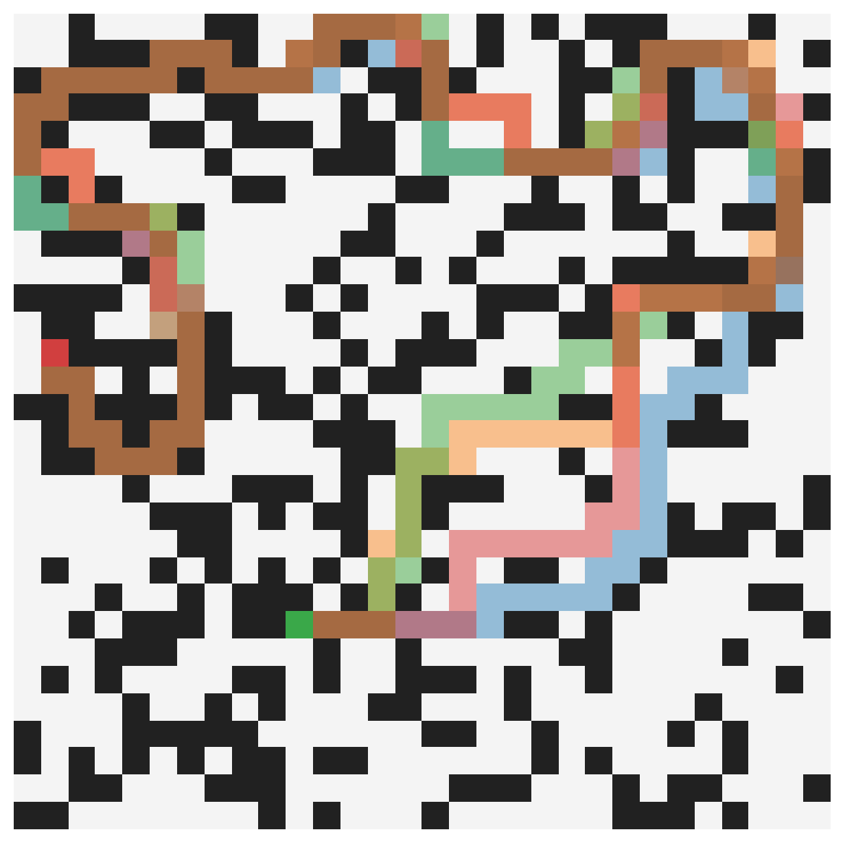
A 30 by 30 Maze-Hard instance drawn as a pixel grid: black cells are walls, light cells are open, with a green start cell and several overlapping coloured paths of equal length winding from start to goal, illustrating that the maze admits many distinct shortest paths. — A single Maze-Hard instance admits millions of distinct shortest paths of equal length, shown here as several overlapping coloured routes — which is why the multi-solution target can sample K of them (LDT, Figure 4).

But the paper is upfront that neither maze setting is empirically sound: the unsolved instances emitted incorrect solutions rather than abstaining. The incorrect answers are still valid paths from start to goal — just slightly longer than optimal. The difference from Sudoku is structural. A Sudoku cell's candidate set going empty is an unmistakable, local $\bot$ ; "this path is one step too long" is a global, numeric property the per-cell lattice does not cleanly represent, so the conflict head has nothing crisp to fire on. The maze is where LDT's multi-solution machinery shines — a 30×30 maze has millions of equally-optimal paths, so the $\alpha$ operator can supervise against a set of sampled solutions ( $K{=}512$ costs only about 2% more per step than $K{=}1$ , reported) — but it is also where the soundness guarantee quietly does not apply. Read the "correct-or-abstain" claim as a Sudoku claim.

Checking the headline: the authors' own correction

The paper's Sudoku-Extreme row says 100%. The released code says otherwise, in a note the authors added themselves:

This is the honest version, and it is more interesting than the round number. The system is neurosymbolic but still built on stochastic ML — not a deterministic solver — so rare failures are expected, and 99.96% is roughly one failure in 2,500 hard puzzles (reasoned, $1 - 0.9996 = 0.0004$ ). The conflict head that lets the model abstain is learned, not proved, which is why the soundness is empirical rather than guaranteed — the asterisk the widget above is honest about. The real claim is narrow but startling: an 800K-parameter model solves 99.96% of search-requiring Sudoku, is wrong essentially never, and gets there in minutes — just not a logic-solver's clean 100%.

The counterpoint: is it searching, or predicting?

A follow-up paper, Anatomy of a Sound Neural Reasoner (arXiv 2607.19635, Aleksey Komissarov), argues that on clue-rich Sudoku the search is largely theatre. The claim, stated fairly: one forward pass already commits essentially the entire grid — every blank cell on standard 6×6, and 94–96% of cells on augmented 9×9 — so the "iterative solver" is really a one-shot predictor wrapped in an exact verifier (reported, critique's abstract). All of the hard-slice failures are decided before search even begins, at the moment the first pass confidently deletes a value the true solution needs — a failure mode the author names first-pass poisoning. Adding the full apparatus of learned branching, minimum-remaining-value heuristics, backtracking, value exclusion and shared nogoods does not change which instances get solved; it cuts repeated invalid derivations by a factor of 1,497 (reported). In other words: the search makes the solver vastly more efficient without making it more capable, because capability was already decided in pass one.

The critique also offers two constructive fixes that are telling. Digit-permutation augmentation on a symmetry-disjoint split lifts 9×9 accuracy from below 1% to 96.5% across three seeds; and a test-time union over symmetry-transformed passes lifts the hard-slice checkpoints from the low-to-high 70s to 100% without any retraining (reported). If search were doing the work, neither symmetry trick should matter that much. The honest synthesis — which the critique itself draws — is that it is a question of regime: on clue-rich completion, accuracy is set by calibration and symmetry and search mostly removes waste; but on a from-scratch graph-coloring task, the one-shot behaviour disappears and search genuinely changes accuracy. So LDT's loop is doing real search somewhere; the debate is whether clue-rich Sudoku is where.

This rhymes with Lanyon's neurosymbolic soundness story: both get their reliability from a hard verifier bolted onto a neural proposer, and in both the useful question is how much the neural part really reasons versus pattern-matches into a space the verifier polices. It is the familiar shape from the looped-transformer literature too — the same tension the compute-matched looping analysis raised, where an impressive headline rests on an accounting choice (there, parameters-not-FLOPs; here, search-vs-one-shot) a careful reader has to unpick.

The take

Strip it to what is defensible and it is still a good result. An 800K-parameter model whose carried state is a sound, typed lattice clears search-requiring Sudoku that trillion-parameter LLMs score zero on, trains in minutes, and — on Sudoku — abstains instead of answering wrong. The mechanism is clean, the soundness-by-asymmetric-loss idea is reusable, and the lattice formulation is domain-agnostic: any abstract domain with a sound deduction operator could be dropped in.

Hold three things loosely. The 100% is really 99.96% on the full test set, by the authors' own correction, and the soundness is empirical, not proved. The soundness guarantee is a Sudoku property — the maze variant is not empirically sound and emits wrong (suboptimal) answers. And the critique's question is open: on clue-rich puzzles the "search" may be one confident forward pass plus a verifier, a different and less general claim than "a transformer that learned to search." The authors concede the honest frontier themselves — a naive port to ARC-AGI, where each task carries its own rules to infer, plateaus at about 36% with no gains from test-time search, because the conflict head becomes unreliable and search cannot tell good branches from bad. That is the real test of whether this is learned search or amortized prediction.

What it clearly is: a reminder that for problems with crisp logical structure, the right representation of the intermediate state — a lattice you can narrow soundly — can beat orders of magnitude more parameters spent emitting tokens into a stream that cannot take anything back.

Sources: Lattice Deduction Transformers (Davis, Haller, Alfarano, Santolucito, 2026) and its released code at github.com/lcrh/lattice-deduction-transformers (MIT, a curated reconstruction); the 99.96% correction is from that repo's README.md and the authors' follow-up thread. The counterpoint is Anatomy of a Sound Neural Reasoner (Komissarov, 2026). Figures 1, 2 and 4 are reproduced from the LDT paper; the 4×4 solver is my own illustration of the solve loop.