Looking Ahead: teaching a chunk-by-chunk video model to predict two seconds out

AK posted it on 22 October with a one-line pitch: "Looking Ahead: Modeling Future Evolution in Autoregressive Video Generation". The replies asked the obvious question: how long does a clip hold together before it falls apart? The first author answered more modestly than the replies did. He called it "a proof-of-concept study" whose data and training pipeline are "at an early stage".

That is the right frame. The paper (Gao, Huang, Hu, Wang, Hu, Shan and Wang; Nanjing University, Tencent ARC Lab and Zhejiang University; 21 October 2026) is not a long-video paper. It is a training-objective paper. It adds one auxiliary loss, Future Chunk Prediction (FCP), to the plain teacher-forced training of a chunk-by-chunk video diffusion model. The claim is that this loss makes the generated physics more plausible and the model's features more structured. It changes nothing at inference.

I read the paper, cloned TencentARC/Looking-Ahead at commit 210794c (22 October 2026) and read the configs, the FCP branch and the loss. I also read the file listings of the released weights on Hugging Face. I did not run anything. The smallest checkpoint is 5.7 GB, the code targets an H200 with CUDA, and no piece of it does anything useful on a CPU. Every result number below is reported unless I say otherwise.

The shortcut inside teacher forcing

Start with the generator. An autoregressive video diffusion model cuts a clip into $K$ chunks of a few latent frames each and factorises the video as

where $\mathbf{c}$ is the text prompt. Each factor is a flow-matching model. Mix the clean chunk with Gaussian noise along a straight line, $\tilde{\mathbf{x}}_{k,t} = (1-t)\,\mathbf{x}_k + t\,\boldsymbol{\epsilon}$, and train a network $\mathbf{v}_\theta$ to predict the velocity $\boldsymbol{\epsilon} - \mathbf{x}_k$. Under teacher forcing the history is the real, clean video:

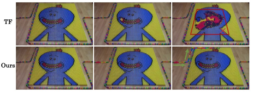
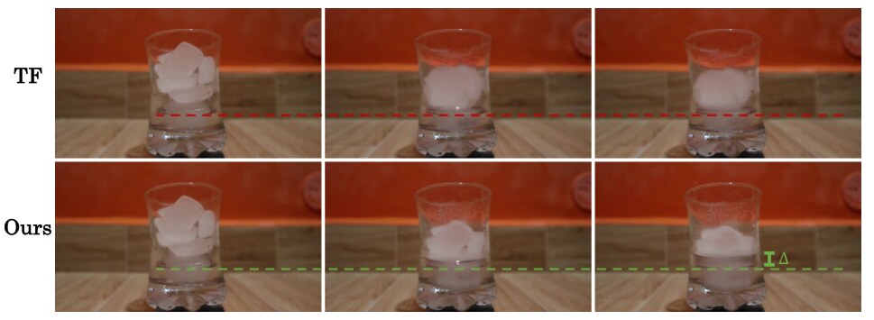
The authors' argument is about what this loss lets the network get away with. Neighbouring chunks of a real video look almost the same: same objects, same lighting, motion that barely changes over half a second. A network that has the clean previous chunk in its context can denoise the current one largely by continuing it. That is a correct answer, and it is cheap. Nothing in the loss forces the network to represent why the scene changes: that the dominoes fall left, or that the water rises as the ice melts.

The fix they propose is to ask a question the previous chunk cannot answer: what does the video look like two seconds from now? The farther out the target, the less local continuity helps. And the target comes free with every training clip, with no external encoder to align to.

Future Chunk Prediction

Formally, FCP keeps the same context and moves the target out by $\Delta$ chunks, hiding everything in between:

so chunks $k+1$ to $k+\Delta-1$ never enter the conditioning. Two practical choices turn this into something trainable.

First, the future predictor gets its own parameters. The authors report that sharing the generator's weights between ordinary denoising and masked-context future prediction "degraded temporal coherence" in preliminary runs. But a separate predictor trained on its own would teach the generator nothing. So the predictor reads the generator's intermediate hidden states, and its loss is backpropagated through them into the generator. This is the multi-token-prediction pattern from DeepSeek-V3, moved from tokens to video chunks.

Second, the predictor reads only the hidden states of chunk $k$, not of the whole history, and no text:

Note that $\Delta = 1$ is now allowed. Predicting the very next chunk from $\mathbf{h}_k$ alone, with no history beyond it and no prompt, is already harder than the main task. The total loss adds one term per offset in a set $\mathcal{D}$, averaged over the clean and the noisy source streams (more on those below):

Each predictor is itself a small flow-matching model. It takes a noised copy of chunk $k+\Delta$, a flow time, and the fused features of chunk $k$, and predicts the velocity. At inference every FCP module is deleted and the generator runs exactly as a teacher-forcing model would.

expand

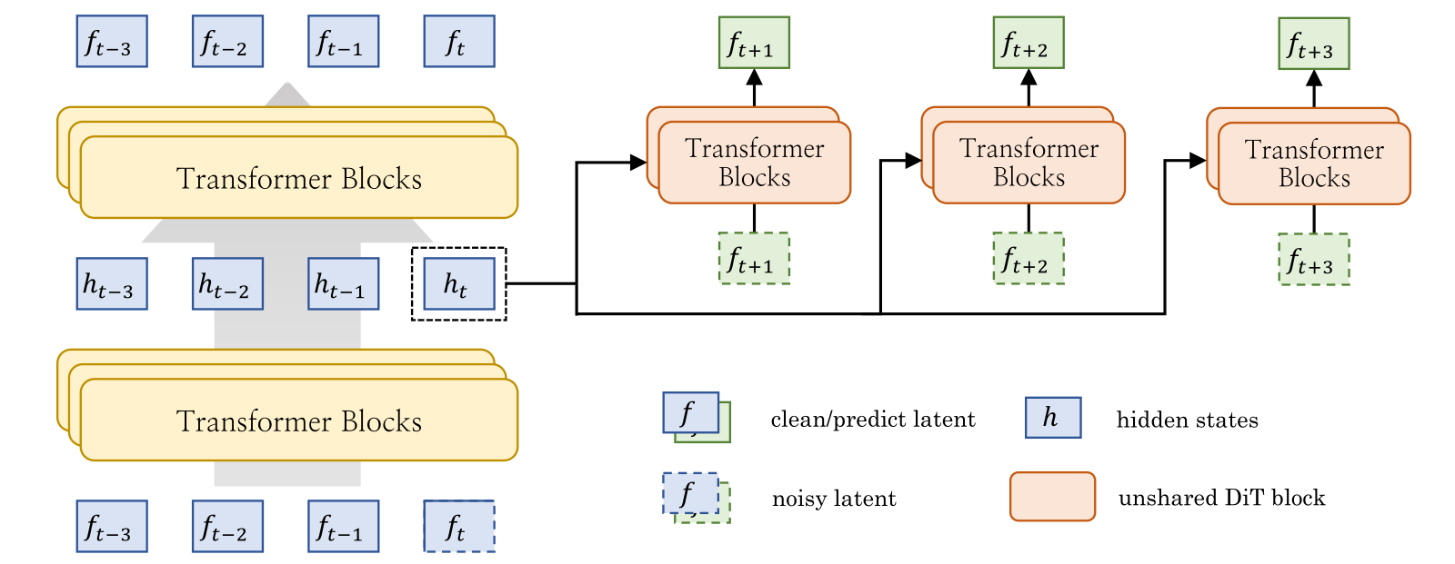
The released configs pin the numbers down. Both generators are initialised from official Wan checkpoints and run image-to-video: the first latent frame is the clean conditioning image, and the rest is cut into chunks of three latent frames. Since a Wan latent frame covers four video frames, a chunk is 12 frames. The 1.3B model trains on 85-frame clips at 16 fps, which is 22 latent frames and 7 chunks, with offsets $\{1,2,3\}$. The 5B model trains on 121-frame clips at 24 fps: 31 latent frames, 10 chunks, offsets $\{1,\dots,5\}$. Every offset weight is 0.5. (Measured from configs/fcp_*.yaml; the chunk arithmetic is mine, which makes it reasoned.)

That gives the horizon in seconds. A chunk is 0.75 s at 16 fps and 0.5 s at 24 fps, so the 1.3B model's farthest predictor looks 2.25 s ahead and the 5B model's 2.5 s (reasoned). The layout code trains every pair $(k, k+\Delta)$ that fits inside the clip, which is $N-\Delta$ pairs for $N$ chunks. That makes 15 pairs per clip on the 1.3B model and 35 on the 5B, each trained twice, once per source stream (reasoned from PredictiveChunkLayout.valid_pair_count).

Pick a source chunk and an offset: the history up to $k$ is visible, the target is $k+\Delta$, and the chunks between are withheld. "Chained" shows the leak described next.

Five design choices, each with an ablation

Clean and noisy sources. Teacher-forced training in this codebase runs the clean chunks and the noisy chunks through the backbone as one sequence; the code concatenates them before the first block. So chunk $k$ has two hidden states: $\mathbf{h}^{\mathrm{clean}}_k$, which later chunks attend to as history, and $\mathbf{h}^{\mathrm{noisy}}_k$, which is being denoised. FCP supervises both, with one shared predictor per offset. On the 1.3B model, supervising only the clean stream lifts Physics-IQ Verified from 27.6 to 28.8, only the noisy stream to 29.9, and both to 30.9 (reported, Table 4).

Parallel, not chained. DeepSeek-style multi-token prediction chains its heads: the head for offset 3 reads the hidden state of the head for offset 2. For diffusion that is a leak. The offset-2 head was fed a partly noised copy of the real chunk $k+2$, so its hidden state carries information about exactly the chunk FCP is trying to hide from the offset-3 head.

expand

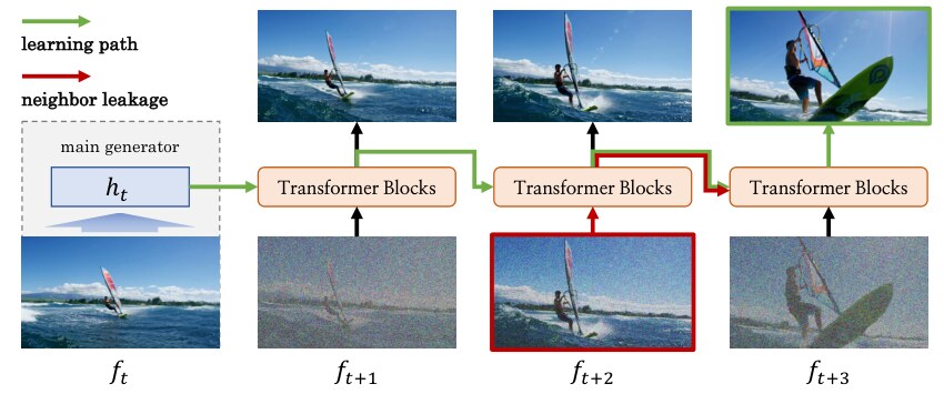
FCP gives each offset its own branch reading $\mathbf{h}_k$ directly. On the 1.3B model chaining costs 0.8 points (30.9 parallel against 30.1 chained). On the 5B model it costs much more. Five chained offsets score 31.0 on image-to-video against 33.8 parallel, and on video-to-video the chained versions fall below the baseline: 39.9 and 40.5 against 40.6 (reported, Table 2). The authors read this as a bigger model being better at exploiting the leak. That is a plausible reading, and one seed-averaged table is not enough to establish it.

No text in the predictor. The predictors drop the cross-attention to the prompt. A prompt such as "the ice melts" is itself a cue about the future, and the point is to make the visual features carry it. Giving the predictor text costs 1.1 points on the 1.3B model (30.9 to 29.8, reported).

Only $\mathbf{h}_k$, not $\mathbf{h}_{\le k}$. This is the main difference from Next Forcing (Xu et al., 2026), which the authors say was developed concurrently. Next Forcing chains its predictors and conditions them on the full history. The paper compares FCP against a full-context variant of itself on the 1.3B model (the compute figure further down) and finds the same plateau at lower cost.

Token-wise AdaLN. Features from four backbone layers are concatenated per token, fused by a two-layer MLP ($4d \to 2d \to d$), and injected into every predictor block as a per-token shift and scale. This is the AdaLN modulation that DiTs normally drive from the timestep, now driven from the source chunk's token at the same position. In the code (PredictiveMultiChunkAttentionBlock) the source projection adds to the timestep modulation, and it is zero-initialised. So at step 0 each predictor ignores the source entirely and must learn to listen. The alternatives score lower: 28.8 for concatenating source and future tokens in one attention, 29.5 for channel concatenation, against 30.9 (reported, Table 7).

What the code adds to the paper

The configs match Table 5. The source layers in the YAML are zero-based: [8, 14, 20, 26] for 1.3B and [2, 11, 20, 29] for 5B. Those are the paper's one-based 9, 15, 21, 27 and 3, 12, 21, 30. The predictors are initialised by copying backbone blocks 17 to 19 (1.3B) and 28 to 30 (5B), as stated. The learning rate, AdamW betas, clipping and step counts (20,000 and 25,000) all match. One mismatch: the paper gives an EMA decay of 0.9995 for the 1.3B run, and both 1.3B configs say 0.999. (All measured.)

The "lightweight" predictors are not light. Each is three DiT blocks without cross-attention. But every block carries its own d → 6d source projection for the token-wise AdaLN. Each branch also has its own fusion MLP, patch embedding, time embedding and output head. Counting parameters from the module definitions with the widths in Table 5 gives 194.2M per branch on the 1.3B model and 710.0M per branch on the 5B (reasoned). Across all offsets that is 583M and 3.55B.

The released weights let me check that count. The FCP checkpoints are larger than their teacher-forcing twins by 2,330,331,037 bytes (1.3B) and 14,200,444,704 bytes (5B), measured from the Hugging Face file sizes. At four bytes a parameter, that is 582.6M and 3,550.1M extra parameters, within 0.01% of the count from the code (reasoned). So the FCP model_ema.pt files ship with the predictors inside: 8.0 GB against 5.7 GB, and 34.2 GB against 20.0 GB. The same arithmetic on the teacher-forcing files gives generators of 1.42B and 5.00B parameters. During training, then, the side predictors add 41% to the 1.3B model's parameters and 71% to the 5B's (reasoned).

They do not run over the whole sequence, and they are thrown away at inference. But "lightweight" undersells what a 5B training run with five offsets carries.

One small departure from the text. The paper says "Target noise and flow time are resampled for each auxiliary prediction". In predictive_fm.py the flow time is resampled per offset. The noise is sliced from the same noise tensor that the main loss uses for that chunk. So a chunk that is the main target and also a future target shares one $\boldsymbol{\epsilon}$ at two noise levels (measured by reading; I did not run it). I doubt it matters much. It is still not what the sentence says.

The results, checked against the tables

The benchmark is Physics-IQ Verified: 198 real videos of physical events. A model sees the start of each (one frame for image-to-video, up to three seconds for video-to-video), generates five seconds, and is scored on how well its motion matches what really happened. IQ is the overall score. SP, ST, WS and MSE are sub-scores that the paper does not define. In the original Physics-IQ benchmark they are spatial IoU, spatiotemporal IoU, weighted spatial IoU and MSE of where motion happens. Every number is the mean of four seeds; the paper gives no spread.

The controlled comparisons hold up as described. On the 1.3B model FCP goes from 27.6 to 30.9. On the 5B model it goes from 30.4 to 33.8 for image-to-video and from 40.6 to 44.4 for video-to-video (reported). The project page's "+11.2%" is 3.4 / 30.4 (reasoned, checks out).

Switch the ledger to the 5B image-to-video set and to the sub-scores, and the gain has a shape. ST rises from 32.8 to 41.1. SP rises 2.0 and WS 1.2, and with three offsets SP and WS are actually below the baseline (33.6 and 23.2 against 34.8 and 24.0). On the 1.3B model ST again moves most: 25.5 to 29.6. So the model gets better at when and where things move across the five seconds more than at the final layout (reasoned from the reported sub-scores). That fits a loss whose whole job is to make features predict later chunks.

expand

expand

The cross-model table needs a caveat the paper half-gives. Table 1 places the 5B FCP model at 33.8, above Wan2.2-14B (32.2), HunyuanVideo-1.5 (33.4), Cosmos3-Nano (29.1) and every autoregressive model listed. Only Grok Imagine Video (34.8) scores higher. But look at the same family. The bidirectional Wan2.2-5B checkpoint they start from scores 24.9, and their own teacher-forced autoregressive fine-tune of it scores 30.4. Of the 8.9 points between the base model and FCP, then, 5.5 come from the autoregressive fine-tune on their data and 3.4 from FCP (reasoned). The base model was run at 1280×704, its native size, while the fine-tunes ran at 1024×576. The authors say the base scored lower when they tried 1024×576. They say plainly that cross-model gaps should not be read as method gaps, and they are right to.

The other physics benchmarks move less. On WorldModelBench the total goes from 7.22 to 7.64. On PAI-Bench-G the domain score goes from 81.13 to 82.38. On PhyGround physics goes from 2.75 to 2.80 (reported, Table 3). All three use a vision-language model as judge, and the authors suggest such judges are less sensitive to the timing of physical changes. That may be true, and it is also what one would say about a small effect.

The compute claim

The abstract says FCP achieves its gains "with a lower overall training compute budget". Here is the figure behind that.

expand

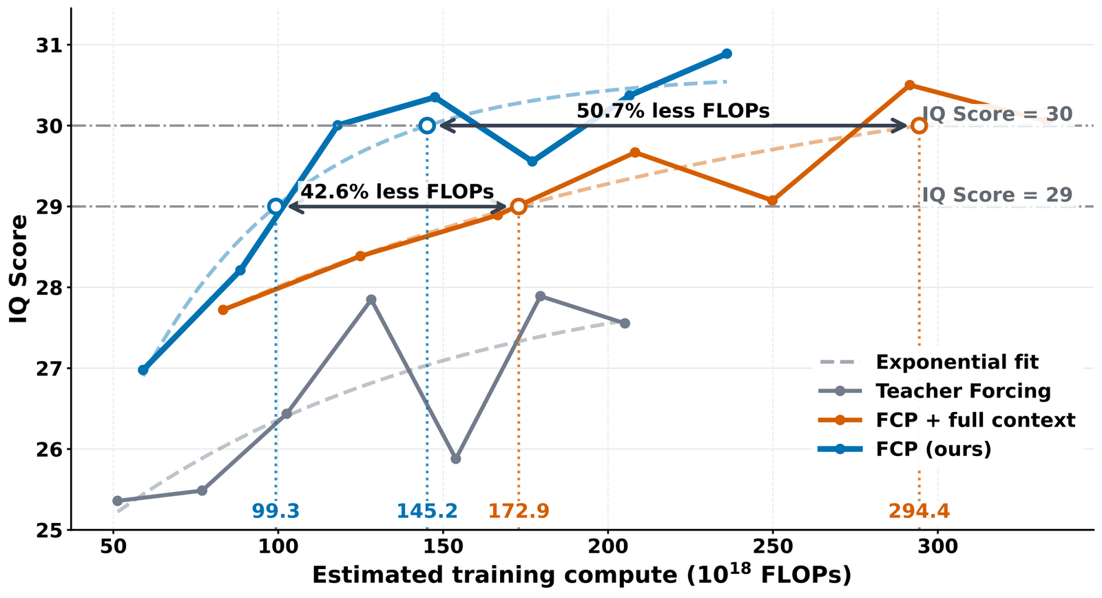
The two percentages check out against the plotted points. Reaching IQ 29 takes 99.3 against 172.9 units, which is 42.6% less. Reaching IQ 30 takes 145.2 against 294.4, which is 50.7% less (reasoned). But both are comparisons between FCP and its own full-context variant, on the 1.3B model only. Against plain teacher forcing the figure supports a different statement: at any matched compute, FCP sits higher. That is a fair "gains do not come from extra compute", not a lower budget.

The figure also shows that FCP costs more per step. Its curve ends at about 236 units and teacher forcing's at about 205, read off the plot. If both curves end at the 20,000 steps both configs set, which the paper does not state, the side predictors add roughly 15% per step on the 1.3B model (reasoned). There is no equivalent figure for the 5B, whose five offsets and 3.55B side parameters should cost proportionally more.

What the predictors see

The side predictors are not meant to be used, but the authors sampled from them anyway. With the generator fed real history, each branch denoises a future chunk from pure noise using only $\mathbf{h}_k$: no intervening frames, no prompt.

expand

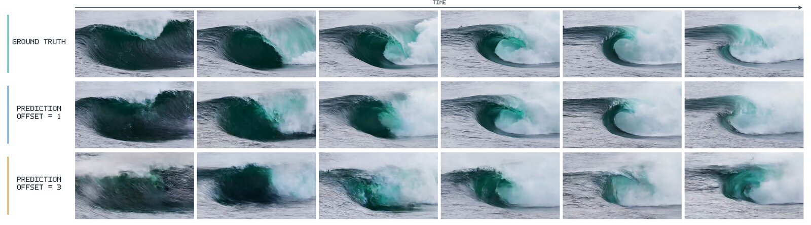
Offset 1 is close to the real wave. Offset 3 loses detail but keeps the motion. That is direct evidence that $\mathbf{h}_k$ carries information about the next second or two of the scene, which is the paper's thesis. The authors float using the branches as cheap drafts for early, high-noise denoising steps. That idea is untested.

The paper also shows token-similarity maps in which FCP features hug the queried object across frames. The query positions were "manually selected" and nothing is quantified, so I read them as illustration.

Where it sits

The site has covered three neighbours of this idea. NextLat does the language-model version: a transformer is trained to predict its own next hidden state, so that the state summarises the past. FCP predicts future data (latent video chunks) from a hidden state, not a future hidden state. LongLive-Plug is the other branch of autoregressive video work. It distils few-step sampling and long-context fixes into plug-in adapters, the rollout-side work (Self Forcing and its descendants) that this paper explicitly does not touch. Matrix-Game 4.0 shows where a causal Wan2.2-5B fine-tune ends up when it must run in real time. Looking Ahead's sampling is 50 UniPC steps per chunk with classifier-free guidance, nowhere near that.

Against that background the contribution is narrow and clean. Diffusion Forcing changes the noise on the history; Self Forcing changes where the history comes from. REPA and VideoREPA align features to a frozen external encoder. FCP leaves the history, the rollout and the encoder alone, and adds a loss whose target is simply a later piece of the same training video. That makes it composable with all of them. Nobody has tested that composition yet: every baseline here is plain teacher forcing with no distillation.

Table 1 has one data point on that interaction. Causal Forcing's teacher-forced Stage 1 checkpoint scores 19.2, and its final, distilled few-step model scores 12.1 (reported). Rollout distillation cost seven points of physical plausibility on this benchmark. Whether FCP's gain survives distillation is the question that decides whether it reaches a real-time model.

Limits

• Five-second clips. Training uses roughly the first five seconds of each video; evaluation generates five seconds. The farthest predictor looks 2.5 s ahead. The question from the replies, whether this keeps long rollouts from drifting, is not addressed. The paper's own limitations section says longer horizons and larger scales are future work.
• Fine-tunes of bidirectional models. Both generators start from bidirectional Wan checkpoints. The authors report that the conversion itself degraded early performance, and suspect it limits what FCP can show. From-scratch autoregressive pretraining with FCP is untested.
• No variance. Four seeds are averaged and no spread is given. Several ablation gaps are about one point on 198 samples.
• Data. Training mixes WISA-80K with internally sourced video that will not be released. The Hugging Face dataset is a demo of pre-encoded latents, so exact reproduction is not possible, as the reproducibility statement says.
• Hardware. The README was tested on one H200. Training used 8 GPUs (1.3B) and 32 GPUs (5B). The FCP checkpoints carry the training-only predictors, so a user who only wants to sample downloads 34.2 GB for a 5B generator whose own weights are 20.0 GB of it.

Licence and release

The code and all four checkpoints (teacher-forcing and FCP, at 1.3B and 5B) are Apache-2.0. The NOTICE credits Wan2.1 and Wan2.2 (Apache-2.0), diffusers schedulers, a T5 encoder from transformers and FramePack memory helpers. The base Wan weights are downloaded separately. The paper is CC BY 4.0. The project page's sample videos carry no stated licence, so this page shows stills from the paper only.

The idea fits in a sentence: make the current chunk's features predict a later chunk, without the chunks in between or the prompt. The controlled results say it is worth three to four points on the main benchmark. The code says it costs more side parameters than "lightweight" suggests. And the gain is mostly in when things move, the part of physics a next-chunk shortcut was most likely to skip.