2026-10-23 · 19 min · 3d · representation-learning · computer-vision · audio · benchmarks · reproducibility
A 1:51 narrated explainer, drawn in code. Every number and picture in it is this article's own; the sources are below.
› transcript
Hi, I'm Soffit! Here is how one small change to an activation helps a network draw sharp edges. A coordinate network turns a position into a value. Earlier fixes chose its frequencies. This one learns how each neuron mixes them. Fourier features, SIREN and FINER change the menu. Each neuron still emits one fixed waveform, welded to its feature. Here the weights still pick the feature. A short list of learned numbers decides the waveform. Here is the formula. It starts as the identity, so the network begins almost linear. Then it adds whole-number harmonics of the same input. Each harmonic gets a learned amplitude, shared by the whole layer. A coordinate goes through the weights, which choose what this neuron looks at. The same value is fed to a bank of sines, one per harmonic. Learned amplitudes weight and sum them, so one neuron can make a square edge on its own. The output is linear in those amplitudes, so tuning the spectrum is a direct problem. In the paper's toy test, SIREN and FINER need more atoms to fit a wiggly signal. The learned harmonic unit fits it with one. The target suits it, so this shows the mechanism. On twenty four Kodak photos the paper reports about thirty eight decibels, just ahead of FINER and three ahead of SIREN. The parameters are almost free. The compute is not: a step takes nearly seven times as long as FINER's. The idea to keep: give each layer a learned recipe for mixing harmonics, and let the weights just pick features. Frequencies picked. Harmonics mixed. Better fits, slower steps. Every source is in the full article. I'm Soffit. Bye!
Why read this
Hightop 30%LSA's harmonic activation from the code up, paper tables rechecked, and a CPU run pricing its per-step lead against wall time.
- Original analysis
- Runs on a consumer GPU
- A lasting reference
3D & spatialNo licenceResearch paper
How this was scored
- Is it new?
- 2 of 3: A real new idea, method or capability
- Can I trust it?
- 2 of 3: Measures key facts from files, code or configs
- Can I run it?
- 2 of 3: Open code or weights with real limits
- Will I understand it?
- 2 of 3: Mechanism from first principles with figures
- Can I act on it?
- 2 of 3: A concrete recipe, numbers or comparison
- Will it last?
- 2 of 3: A reference for a year or more
- Does it affect many?
- 1 of 3: A specialist community
- Only here?
- 2 of 3: A teardown or measurement few others did
Score 67 of 100, ranked 178 of 607 rated articles. Each question is answered 0–3 by hand, and a 3 is rare. How articles are scored
An implicit neural representation (INR) stores a signal as a function. Give a small MLP a coordinate (a time stamp, a pixel position, a point and a view direction) and it returns the value there (an audio sample, an RGB triple, a density and a colour). There is no grid. You can query it between samples, take its derivative analytically, and optimise through it. NeRF is the famous instance; signed distance fields, like the one inside OREN's octree mapper, are another.
The catch is old and well known. A plain ReLU MLP fed raw coordinates learns smooth functions first and fine detail last, sometimes never. That is spectral bias: gradient descent fits the low-frequency part of the target much faster than the high-frequency part. A photo through a ReLU MLP comes out blurry, and an audio clip comes out as mush.
Learnable Spectral Activations (LSA), by Tamir Shor, Or Litany and Alex Bronstein (Technion, NVIDIA, ISTA), arXiv 2610.07419, NeurIPS 2026, comes with code. Litany's pitch on X: prior INR work tunes which frequencies are available; LSA learns how to compose them. Below: what that means for one neuron, the tables checked against the paper and code, and a small CPU run.
- branch
- HEAD
- tests
- none found
- source
- 82.9 kB
- commit date
- 2026-10-07
by size of tracked source at this commit, file counts in brackets; docs, data and vendored trees excluded
local clone, 2026-10-23 at 35a040b — branch, commit, commitDate, fileCount, hasTests, languages
Every fix so far changes the frequency menu
The cleanest way to read INR design is the structured dictionary view of Yüce et al. (2022), which the paper adopts. Feed a network a sinusoid of frequency , push it through a nonlinearity , and you get harmonics: . Stack layers and the network's output is a weighted sum of sinusoidal atoms whose frequencies come from a set the architecture induces:
Read the popular fixes through that lens and they all edit the menu:
- Positional encoding / Fourier features (NeRF; Tancik et al.) prepend . The matrix is the base frequency set. With random , is a bandwidth knob: larger exposes higher frequencies and risks aliasing between samples.
- SIREN uses as the activation, with . sets the bandwidth the network can resolve.
- FINER uses : the local frequency grows with the magnitude of the pre-activation, so the bias initialisation picks which frequencies are reachable.
- WIRE, sinc activations and learned initialisations change the atoms' shape or where training starts.
The paper's argument is that all of these decide which atoms exist and leave the neuron's own waveform prescribed. A SIREN unit's output is : one sinusoid of the projection . Its harmonic content is fixed by the same weights that choose which feature the unit looks at. To build an edge, which needs many harmonics in fixed amplitude ratios, the network has to recruit several such units and line them up. The waveform and the feature are welded together.
The activation
LSA unwelds them. At hidden layer the activation is a residual, truncated Fourier series of the scalar pre-activation (paper, Eq. 2):
- is one neuron's pre-activation.
- is the number of harmonics: 16 for audio, 32 for images, 24 for NeRF and 8 for the acoustic fields.
- are learnable and shared by every neuron in the layer, so a layer adds parameters, not width.
- The leading is a residual identity. The coefficients start near zero (standard deviation 0.01 for audio, for images), so the network begins as an almost linear MLP and grows its nonlinearity during training.
Three properties fall out of the form.
The waveform is decoupled from the feature. still decides what the unit looks at. The coefficients decide what it does with it: the same goes through harmonics at once, and their relative amplitudes are learned. One unit can emit a square-ish wave, a sawtooth, or something with a notch.
It is affine in the coefficients. For fixed pre-activations, is linear in . The gradient for is the residual's correlation with the propagated harmonic . The paper writes this as an exact finite-width identity for full-batch gradient flow (Eq. 4):
where is the residual, the Jacobian with respect to ordinary weights and the Jacobian with respect to the harmonic coefficients. The second term is extra descent the coefficients add whenever the residual has any projection onto the harmonic directions. Equivalently, the empirical neural tangent kernel gains a positive semidefinite term of rank at most (layers ). That is the formal content of "spectral tuning becomes a more direct subproblem".
It does not expand what the network can represent. The paper is careful here and I will be too: a wide enough periodic INR can already represent the same signals. LSA changes the factorisation, not the function class. The claim is about optimisation: the same target is easier to reach.
The widget below is one LSA activation with . Left: against the identity it starts from and against a single sine. Right: its spectrum, which for this form is just the coefficient vector, one bar per harmonic. A SIREN unit has one bar.
The fit edge button makes the affine point concrete. The target is a soft square wave, , added on top of . Because is linear in , the best coefficients are a least-squares solve, not a search. The best root-mean-square gap with only the first harmonic, which is all a single sine can do, is 0.155 against a target RMS of 0.431. Adding harmonics two and three brings it to 0.089, and five or six bring it to 0.057 (measured, in the widget and in numpy). The even harmonics get zero weight: the target is an odd square wave, and a square wave has no even harmonics. A SIREN or FINER network gets there too, but by recruiting more units at different frequencies and phases, which costs width and gradient steps.
The paper's own version of this is Figure 1a: a 1D target fitted with a budget of one to four atoms.
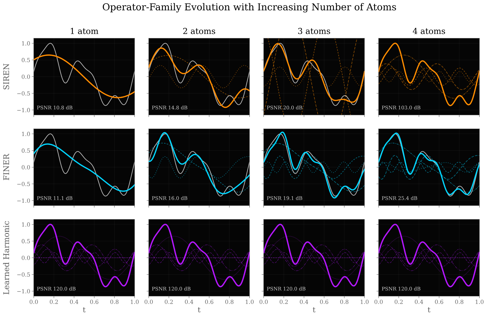
Take the 120 dB with a grain of salt. The phantom appears to be built from a few harmonics of one fundamental, which is the one case where a single learned-harmonic unit is an exact fit (reasoned from the figure; the paper does not give the phantom's formula). It shows the mechanism, not a margin.
What the released code actually does
The repository ships the audio and 2D image experiments only. NeRF and the
neural acoustic fields are not in it (measured, at commit 35a040b, 7 October
2026). It also has no licence file. The THIRD_PARTY.md lists the FINER, STAF
and SL2A sources, and the STAF and SL2A licences are kept, but the repo itself
grants nothing, so treat it as all rights reserved until that changes.
The image activation in image_2d/lsa/models.py is ten lines:
class SpectralActivation(nn.Module):
    def __init__(self, harmonics=32, init_scale=1e-3, residual=True):
        super().__init__()
        self.harmonics = int(harmonics)
        self.residual = bool(residual)
        self.coeffs = nn.Parameter(init_scale * torch.randn(self.harmonics))

    def forward(self, x):
        y = 0.0
        for i in range(self.harmonics):
            y = y + self.coeffs[i] * torch.sin(2.0 * math.pi * (i + 1) * x)
        return x + y if self.residual else y
Two details matter that the equations do not show (measured from the code):
- The forward pass is a Python loop over . Every harmonic is a separate
sin, a separate multiply-add and a separate saved tensor for autograd. That is the cost the paper's resource appendix measures, and the cost my CPU run hits. - The first layer has no . Its weights and biases are uniform in (that is, with two input coordinates), and the activation multiplies the pre-activation by for up to 32. So the first LSA layer is, in effect, a Fourier-feature bank along each neuron's direction , with frequencies up to and amplitudes learned per layer (reasoned). Hidden layers use SIREN's initialisation bound, . The harmonic basis is where the high frequencies come from, which sits a little awkwardly next to "LSA does not change which frequencies are available". It does not change the asymptotic menu; it does change what a finite network reaches from initialisation.
The training loop puts the coefficients in their own Adam group at a higher
learning rate: twice the weight rate for images, three times for audio
(act_lr_mult in image_2d/configs/kodak_core.yaml and audio/run_core.py).
Checking the results
All numbers in this section are reported: the paper's, on an NVIDIA RTX A6000, not re-run. Where I combine them, it is reasoned.
Images: Kodak
Twenty-four 768×512 photos, raw coordinates, width 256, four nonlinear layers, 5,000 Adam updates, seed 0, best PSNR along the trajectory. Mean PSNR:
| Method | Mean PSNR (dB) | Setup |
|---|---|---|
| LSA () | 38.110 | 199,043 params, 5,000 updates |
| FINER | 37.317 | 198,915 params, 5,000 updates |
| WIRE | 36.596 | up to 10,000 updates |
| STAF (global config) | 35.369 | matched budget |
| MFN GaborNet | 35.151 | up to 10,000 updates |
| SIREN | 34.990 | 198,915 params, 5,000 updates |
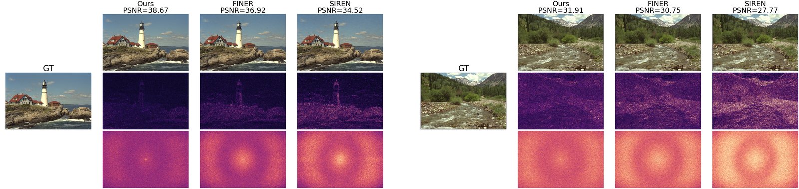
LSA beats FINER on 21 of 24 images and SIREN on all 24. The gap over FINER is 0.79 dB (reasoned). The paper selects LSA's configuration on six calibration images (kodim02, 05, 07, 10, 13, 23); on the other 18, LSA reports 38.045 dB.
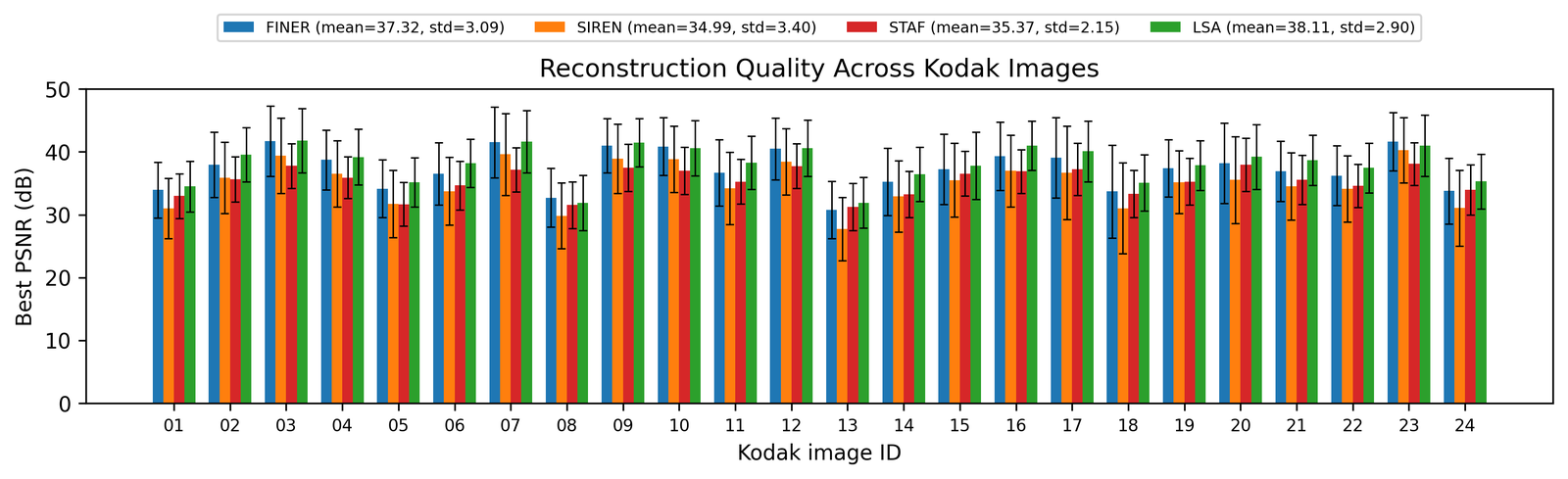
Three things to hold the table to:
- One seed. Every image fit is seed 0. The paired statistics are across images, not across initialisations. With 21 of 24 wins the image-level result over FINER is not noise, but the 0.79 dB is a one-seed number.
- The STAF and SL2A comparisons are protocol-sensitive. Against full SL2A the holdout gap is 0.188 dB with ten wins and eight losses; the paper's own sign test gives . Against SL2A at matched parameters (199,171) the gap is 2.135 dB and LSA wins all 18. So "LSA beats SL2A" depends on which SL2A.
- The ablations are informative. gives 30.45 dB on the six calibration images, gives 39.50 dB and gives slightly less. Freezing the coefficients at their near-zero initialisation drops held-out PSNR from 38.05 to 19.91 dB. That second number is not "LSA versus a fixed good activation". A frozen near-identity activation leaves an almost linear MLP, which cannot fit a photo at all (reasoned). It proves the coefficients are doing the work, which is the point of the ablation.
Audio: where the gap is largest, and needs Fourier features
One-second clips at 48 kHz, 10 from NSynth and 40 from LibriSpeech, width 256, four layers, 5,000 full-batch updates. Each method gets the same 16 Gaussian Fourier-feature bands at each bandwidth , and the paper sweeps from 0 (raw coordinates) to 100.
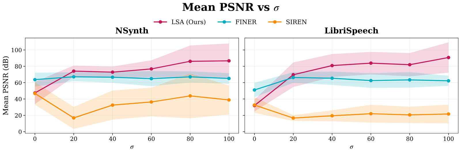
At LSA reports 86.72 dB on NSynth and 90.78 dB on LibriSpeech. The strongest STAF setting reaches 68.79 and 68.40 dB; FINER reaches 67.19 and 66.32 dB. Read three things off the figure before quoting those:
- At FINER wins. With raw coordinates LSA is below FINER on both datasets. The paper says so and explains it: LSA reshapes the frequencies it is given; it does not add a new input basis. The audio win is LSA plus Fourier features against FINER plus Fourier features.
- The spread is large. LSA's 86.72 dB on NSynth carries a standard deviation of 21.18 dB across ten clips; LibriSpeech's 90.78 carries 18.57.
- The absolute numbers are past audibility. 90 dB PSNR on a unit-peak waveform is an RMS error of about , roughly one 16-bit quantisation step (reasoned). Both LibriSpeech and NSynth are distributed at 16 kHz and are resampled to 48 kHz here, so the grid is oversampled three times over. These are memorisation benchmarks. The more useful audio result is the off-grid one: trained on 16,000 samples and evaluated at the midpoints, SIREN with large collapses between samples and LSA does not (paper, Figure 3; the figure gives no table to check).
The released README notes that the core audio targets are zero-mean and unit-peak, while the appendix says amplitudes are used "on the decoded floating-point audio scale". It is applied identically to every method in the core comparison, so it does not tilt the table, but the two descriptions do not match (measured from both files).
NeRF: a tie on PSNR, a small SSIM edge
Blender, eight scenes, FINER's reduced-view protocol (every fourth training image, 200×200), an Instant-NGP-style backbone with width 182, 150,000 steps, final checkpoint. LSA uses .
| Mean over 8 scenes | PSNR (dB) | SSIM |
|---|---|---|
| SIREN | 28.99 | 0.932 |
| FINER | 29.26 | 0.932 |
| LSA | 29.29 | 0.938 |
The means are reasoned from the paper's Table 1. LSA is best on PSNR in five scenes and FINER in the other three; the mean PSNR gap to FINER is 0.03 dB, with Lego going 0.65 dB the other way. SSIM is the more consistent signal: LSA is best on seven of eight scenes. The paper calls these gains "moderate", which is accurate. One run per scene, and LSA's learning rate is three times the baselines' ("best stable settings"), so this is a parity result with a mild structural-similarity edge, not a NeRF upgrade.
Neural acoustic fields
Here LSA () replaces the activation in the NAF decoder and nothing else. Log-spectral L1 improves by 44.90% (macro over four scenes), MRSTFT log-L1 by 45.97% and the interaural time-delay error from 122.4 to 39.7 samples; waveform PSNR improves by 0.43 dB. The largest relative effect in the paper, and the one I can least check: the NAF code is not released, and the baseline (waveform PSNR 11.417 dB) is far from the ground truth.
What it costs
Here the paper is direct. The parameters are free: depth 4 with adds 64 scalars to a 206,337-parameter audio MLP. The compute is not. On full-grid 48k audio fitting with 16 Fourier bands, an A6000 step takes (reported, Table 16):
| Depth 4, width 256 | Train step (ms) | Train peak mem (GB) | Eval (ms) |
|---|---|---|---|
| SIREN | 8.26 | 0.48 | 3.56 |
| FINER | 14.20 | 0.85 | 5.55 |
| LSA, | 97.93 | 7.53 | 35.08 |
That is 6.9× FINER's step time and 8.9× its memory (reasoned; the paper rounds to 7× and 9×). Both scale linearly in : at a step takes 341.09 ms and 29.55 GB. The cause is the one in the code: the activation evaluates batch × width × layers × sines and autograd keeps each one. An "accumulate" implementation cuts inference memory, and the paper points at a fused kernel as future work. The math is a natural fit for one: the derivative of is , and both sums can come from one Chebyshev-style recurrence on and of without storing tensors (reasoned; nobody has shipped it).
The paper leaves quality against wall clock to future work. That is the experiment I could run.
Running it: one image on a CPU
Setup (measured). The released LSAImageMLP and the released SIREN and
FINER classes (image_2d/third_party/finer.py), imported from the clone; my
own training loop mirroring image_2d/lsa/train.py (Adam, learning rate decayed
to 0.1× over the run, LSA coefficients at twice the weight rate, targets in
). A fourth baseline is a ReLU MLP with NeRF-style positional encoding
( octaves, width trimmed to 121 to match parameters). The image is
scikit-image's astronaut (NASA, public domain) at 128×128, full batch.
Width 128, four nonlinear layers, . Every model has about 50,000
parameters. Hardware: a shared 4-core Intel Xeon at 2.10 GHz cloud VM, CPU only,
PyTorch 2.14.1, two threads, nice 19, with other jobs running.
Total compute for the run was about 28 minutes of wall time, over the 20-minute budget I set myself, almost all of it the LSA model.
| 500 steps, ~50k params | Final PSNR (dB) | ms per step | Training time (s) |
|---|---|---|---|
| FINER | 41.66 | 97 | 48.5 |
| SIREN | 37.80 | 82 | 41.0 |
| LSA, | 35.12 | 2,767 | 1,383 |
| ReLU + positional encoding | 24.75 | 50 | 25.0 |
| SIREN, run for 2,000 steps | 48.61 | 92 | 184 |
What the run shows (all measured, one seed, one image):
- At 500 steps LSA is behind, not ahead. 35.12 dB against SIREN's 37.80 and FINER's 41.66, and still climbing when the budget ends. That does not contradict the paper so much as sit at the start of its own curve: the paper reports LSA ahead of FINER on only 5 of 24 Kodak images at step 500, rising to 21 of 24 by step 2,000. I ran a smaller network on a smaller image for a tenth of the steps, with the paper's learning rates rather than tuned ones. It also says I could not reproduce "LSA separates from SIREN early" at this scale: the paper has LSA ahead of SIREN on 23 of 24 images at step 500.
- Per step, the released activation is 26 to 34 times slower than SIREN on
this CPU. 1,614 ms against 62 ms in a quiet ten-step benchmark, 2,767 ms
against 82 ms over the full run with the machine loaded. The paper's A6000
ratio against SIREN is 11.9× (97.93 / 8.26 ms, reasoned); a CPU has no spare
parallelism to hide 32 separate
sinkernels and their saved tensors, and peak memory for the LSA process reached about 4.4 GB against a few hundred MB for the others. - At matched wall time it is not close. SIREN given 2,000 steps reaches 48.61 dB in 184 seconds, under a seventh of the 1,383 seconds LSA spent to reach 35.12 dB. On this hardware and at this size the honest summary is that LSA's advantage, if it arrives, arrives after a cost that a faster activation could spend on more steps.
- The coefficients do move, and the last layer goes flat. After 500 steps the first layer's 32 coefficients are spread between about −0.04 and +0.04 with mixed signs; the last hidden layer's are all close to −0.042, a nearly uniform harmonic profile. The paper's Figure 19 describes the same pattern on Kodak: selective early layers, broad uniform support in the final hidden layer.
- ReLU with positional encoding is the weakest at 24.75 dB. I did not tune ; ten octaves put the top frequencies past this 128-pixel grid's Nyquist limit, so treat it as a floor, not a fair baseline.
Treat this as a smoke test of the released code and a price check, not a
replication. Reproducing the Kodak table needs a GPU, 768×512 images, width
256 and 5,000 steps per fit, and the released image_2d/run_core.py does
exactly that.
Where this leaves LSA
The idea is small and sound: learned, layer-shared harmonic amplitudes cut the tie between a neuron's waveform and its feature for parameters per layer, and give the optimiser clean new descent directions. On images that buys a consistent 0.8 dB over FINER and 3 dB over SIREN at matched width and steps. On audio it buys a lot once Fourier features are present, and nothing without them. On NeRF it buys parity.
What I would want before adopting it:
- A wall-clock comparison. At a fixed GPU-hour, is LSA still ahead of FINER? My CPU run never reached the point where LSA's per-step lead shows up, and the per-step price is large. A fused kernel would change the answer, and does not exist yet.
- Seeds. One seed per image, one run per NeRF scene.
- The NeRF and NAF code. The two field results are the most interesting and are not reproducible from the release.
- A licence on the repository.
Related reading: RoPE applies the same sinusoidal-feature idea to token positions; the Gaussian-splat appearance benchmark is a field where the frequency question moved out of the MLP into spherical harmonics; and functional gradient descent is another way to think about optimising a function rather than its weights.