Pocket TTS with drifting: a one-step speech head without the Jacobian

2026-10-06 · 18 min · tts · speech · audio · generative-models · flow-matching · distillation · on-device · explainer

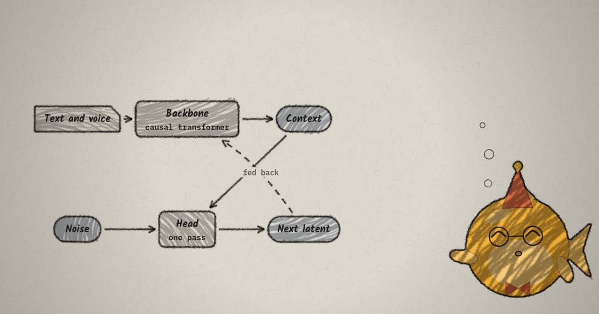
Kyutai's Pocket TTS is a 100M-parameter text-to-speech model that clones a voice from a short prompt and runs faster than real time on a CPU. At its core is a tiny network that has to turn noise into the next 80 ms of audio in one forward pass. On 28 September Kyutai published a technical post on retraining that network with drifting, a one-step generative objective from Deng, Li, Li, Du and He. Their claims: under 1% WER, voice cloning intact, and, as far as they know, the first speech model and the first autoregressive model trained this way.

The interesting part is not the parity. It is that drifting does the same job as their previous objective, LSD, without a Jacobian-vector product anywhere in training. It also needed one ingredient the paper did not have: a kernel temperature that is learned rather than fixed.

I read three things for this: the blog post, the repository at commit 41cbc84 (training/modules/samplers.py holds both losses), and the safetensors headers of the released checkpoints. I did not train or run the model. In what follows, measured means I read it from a file, reported means it is Kyutai's or the paper's figure, and reasoned means my arithmetic on the other two.

Where the one step lives

Pocket TTS is a continuous audio language model (CALM). The Mimi codec compresses 24 kHz audio into one 32-dimensional latent per frame at 12.5 Hz, so one frame every 80 ms (reported; frame_rate: 12.5 and dimension: 32 in english_drifting_26-09.yaml, measured). There are no discrete tokens and no softmax over a codebook. Generation is autoregressive:

A causal transformer reads the voice prompt, the text and the latents so far, and emits a context vector $z_t$ .
A small MLP, the sampler head, maps $(z_t, \varepsilon)$ to the next latent, where $\varepsilon$ is fresh Gaussian noise. The noise is what lets the head draw from a distribution of plausible next frames instead of regressing to their average, which sounds muffled.
Mimi's decoder turns latents back into a waveform.

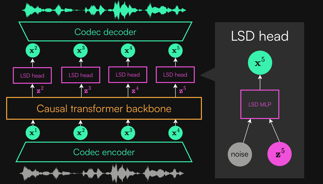
Architecture diagram on a dark background. Audio enters a codec encoder at the bottom, producing latents x1 to x4. A causal transformer backbone reads them and outputs context vectors z2 to z5, each feeding a magenta 'LSD head' box that outputs the next latent x2 to x5. A codec decoder at the top turns these into a waveform. A callout on the right shows one head: an MLP taking noise and z5 and producing x5. — Pocket TTS: a causal transformer emits a context vector per frame and a small head turns noise plus that context into the next codec latent. The post swaps only the objective that trains the magenta head; codec and backbone are unchanged. (Kyutai blog, Pocket TTS architecture figure.)

The checkpoint headers give the sizes. The drifting model english_drifting_26-09 (the no-voice-cloning variant, which is readable without a login) has 108.7M parameters in total: 75.5M in the transformer, 8.97M in the head, and 20.1M in Mimi (measured, summed from tensor shapes). The LSD model english_2026-09 has a 9.76M head (measured). The 0.79M difference is the LSD head's two time embedders: LSD conditions the head on a start and an end time, and drifting has no time at all (num_time_conds = 0 in mlp.py, measured).

At inference the drifting head really is one call. The whole decode function is this (measured, pocket_tts/models/flow_lm.py):

def drifting_decode(v_t: FlowNet, x_0: torch.Tensor, num_steps: int = 1) -> torch.Tensor:
    """One-step head without time conditions: the sample is the head's output for the noise."""
    return v_t(x_0)

Why one step is hard, and what LSD charged for it

The head runs once per frame, 12.5 times a second, on a CPU. A 20-step ODE solver would multiply the head's cost by 20. So the head must be a one-step (1-NFE) generator.

Flow matching on its own does not give you that. It learns a velocity field and needs an integrator at sampling time. The one-step flow objectives (MeanFlow, and the Lagrangian and Eulerian self-distillation family) train the network to jump the whole trajectory in one go. The price is a derivative of the network along its own trajectory. You can see it in Kyutai's LSD loss (measured, samplers.py):

vt, dvdt = torch.func.jvp(
    v_t, (s, t, x_s), (torch.zeros_like(s), torch.ones_like(t), torch.zeros_like(x_s))
)
x_t = x_s + (t - s) * vt
dxdt = vt + (t - s) * dvdt

That jvp is a forward-mode derivative of the head with respect to its time input. The code comment prices it at about two extra head forwards plus their backward. It is expensive enough that Kyutai computes the self-distillation term on only a quarter of steps (distill_prob = 0.25, measured), which the comment says trains about 9% faster. The blog also calls it "numerically delicate". The Jacobian-free alternatives (shortcut models, PSD, consistency models) "trained to a clearly worse model" in Kyutai's hands (reported, no numbers given).

Drifting, from first principles

Diffusion and flow models iterate at inference. Drifting moves the iteration to training. Training is already iterative: every optimizer step changes the network, so it changes every sample the network produces. Call the generator $f_\theta$ and its output distribution $q$ , the pushforward of the noise. If $x_i = f_{\theta_i}(\varepsilon)$ , then after one optimizer step the same noise lands at $x_{i+1} = x_i + \Delta x_i$ . The paper's move is to choose that $\Delta x$ with a field $V_{p,q}$ that depends on the data distribution $p$ and the current $q$ :

x_{i+1} = x_i + V_{p,q}(x_i).

What should $V$ be? It must be zero when $q = p$ , or training would keep pushing a perfect generator. The paper gets this from anti-symmetry: if $V_{p,q} = -V_{q,p}$ for every $x$ , then $q = p$ gives $V_{p,p} = -V_{p,p}$ , so $V = 0$ (Proposition 3.1). The converse is not true in general. The paper offers only a heuristic argument (Appendix C.1) that a near-zero field of its specific form means $q \approx p$ .

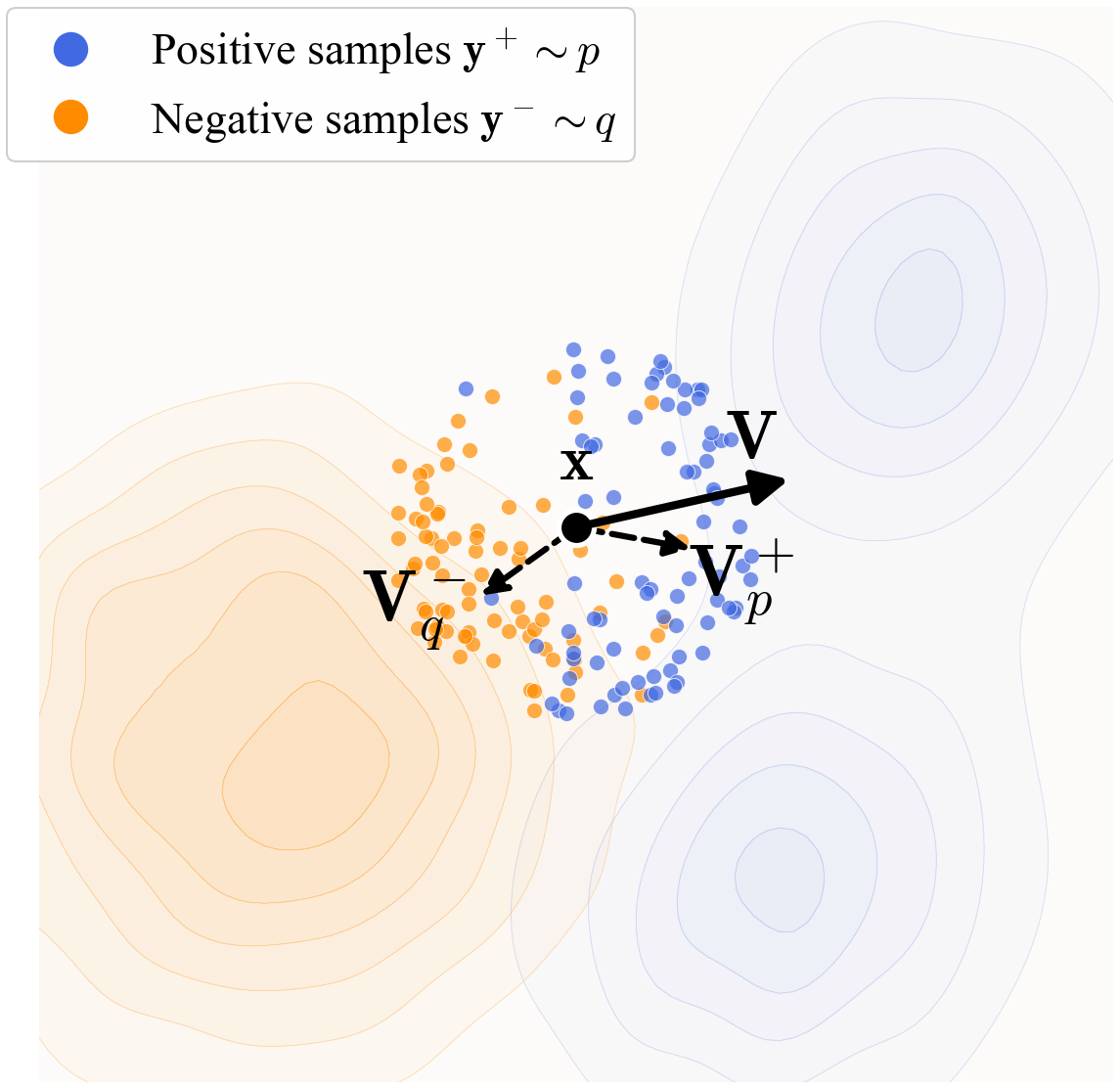
The form they pick is attraction minus repulsion, each a mean-shift vector:

V^{+}_p(x) = \frac{\mathbb{E}_{p}\left[k(x, y^{+})(y^{+} - x)\right]}{\mathbb{E}_{p}\left[k(x, y^{+})\right]}, \qquad V^{-}_q(x) = \frac{\mathbb{E}_{q}\left[k(x, y^{-})(y^{-} - x)\right]}{\mathbb{E}_{q}\left[k(x, y^{-})\right]},

V_{p,q}(x) = V^{+}_p(x) - V^{-}_q(x), \qquad k(x, y) = \exp\left(-\lVert x - y \rVert / \tau\right).

$V^{+}$ points from $x$ to a kernel-weighted average of nearby data. $V^{-}$ points from $x$ to a kernel-weighted average of nearby generated samples, and subtracting it pushes $x$ away from them. Swap $p$ and $q$ and the field flips sign, so it is anti-symmetric. Where generated samples are too dense, repulsion wins. Where data is uncovered, attraction wins. The kernel is Laplacian, $\exp(-d/\tau)$ on the plain Euclidean distance, and $\tau$ is the temperature: the distance over which a sample feels its neighbours.

A scatter plot with blue positive samples drawn from a data distribution on the right and orange negative samples from the generated distribution on the left. A black generated point x has two dashed arrows: V_p plus toward the blue samples and V_q minus toward the orange samples. A solid arrow V, the difference, points further toward the blue data. — One sample's drift. V⁺ is the mean shift toward positives (data), V⁻ the mean shift toward negatives (generated samples), and the sample moves along V = V⁺ − V⁻. (Drifting paper, Figure 2.)

Two frames side by side. Left, at the start: eight blue generated dots bunched together near the top, with two clusters of gold data stars below them, one on the left and one on the right. Right, after drifting: the blue dots have split, four sitting on the left cluster of stars and four on the right cluster. — Kyutai's own picture of the field: generated samples (blue) are pulled to the data (gold) and pushed apart from each other, so they split across both clusters instead of piling onto one. Two frames of the post's looping animation, at its start and at 6 s. (Kyutai blog, drifting field figure.)

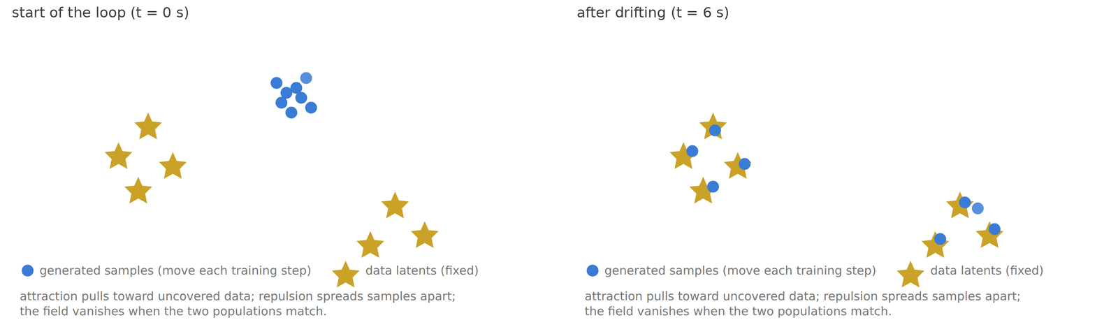
The training loss turns the update into a regression on a frozen target:

\mathcal{L} = \mathbb{E}_{\varepsilon}\left\lVert f_\theta(\varepsilon) - \operatorname{stopgrad}\left(f_\theta(\varepsilon) + V\left(f_\theta(\varepsilon)\right)\right)\right\rVert^2 .

The value of this loss is just $\mathbb{E}\lVert V \rVert^2$ . Its gradient with respect to the output $x = f_\theta(\varepsilon)$ is $2(x - (x + V)) = -2V$ . So a gradient-descent step moves each output along $+V$ , and back-propagation spreads that move into the weights. There is no trajectory, no time variable and no second derivative. You never differentiate through $V$ itself, because the stop-gradient freezes it. The network only needs a forward pass and an ordinary backward pass.

The anti-symmetry is load-bearing. The paper's Table 1 breaks it on purpose: the balanced $V^{+} - V^{-}$ reaches FID 8.46 on its ImageNet ablation model, 1.5x attraction gives 41.05, 1.5x repulsion gives 46.28, and attraction alone gives 177.14 (reported). Attraction alone is mode-seeking regression; repulsion is what spreads the samples.

Eight small scatter plots across the top: orange generated samples at training iterations 0, 50, 100, 200, 500, 1000 and 2000, starting as a small blob, spreading into a square, and resolving into a checkerboard pattern that matches the blue ground-truth checkerboard on the right. Below, a loss curve on a log scale falls steadily over 2000 iterations. — A small MLP generator drifting toward a 2D checkerboard: the samples start as a blob, spread, then resolve the pattern, while the loss (the squared field) falls. (Drifting paper, Figure 4.)

What the shipped loss computes

The blog's pseudo-code uses two separate softmaxes, one over the data and one over the siblings. The code in Drifting._drift is the paper's Algorithm 2 instead (measured). Per frame it takes the $N$ generated candidates and computes the distances from each one to [data sample, the other N candidates]. It divides those distances by their mean for that frame, and forms logits $-d/\tau$ . Then it normalises those logits two ways, a softmax over targets and a softmax over candidates, and takes their geometric mean:

A = (logit.softmax(dim=-1) * logit.softmax(dim=-2)).clamp(min=1e-6).sqrt().detach()
A_pos, A_neg = A[..., :1], A[..., 1:]
W_pos = A_pos * A_neg.sum(dim=-1, keepdim=True)
W_neg = A_neg * A_pos.sum(dim=-1, keepdim=True)
force = W_pos @ y_pos - W_neg @ y_neg

Pocket TTS has exactly one positive per frame. With one positive, the weight sums are equal: $\sum W_{\text{pos}} = A_{\text{pos}} \sum_j A_{\text{neg},j} = \sum_j W_{\text{neg},j}$ . So the code's correction term (W_pos.sum - W_neg.sum) * x is zero. The field reduces to

V(x) = \sum_j A_{\text{pos}}\, A_{\text{neg},j}\,\left(y^{+} - y^{-}_j\right)

(reasoned). This is the paper's Eq. 11 with an empirical estimate: every sibling contributes a vector pointing from itself to the data sample. It is weighted by how strongly $x$ feels both of them. A candidate with no sibling nearby and no data nearby gets almost no push. Remember that, because it is the failure mode the temperature fixes. The drift is then divided by its RMS, averaged over the batch (normalize_force="batch", as in the paper). Each candidate's distance to itself gets 100 added after normalisation, so it never attracts or repels itself.

The temperature is the whole game

Here is the knob in a toy. The rules are exactly the code's: per-frame normalised distances, the double softmax, $W_{\text{pos}}$ and $W_{\text{neg}}$ , and samples that move by the field. There is no network, so the samples move directly. That move is the one the loss asks the network to make. The data has three clusters and many positives, unlike Pocket TTS's one, so this shows the kernel's geometry, not Kyutai's training run.

kernel temperature

τ = 0.306training step 160 / 160

τ at this step: 0.306
miss (data → nearest sample): 0.22
sample spread (data: 3.34): 3.70
field RMS: 0.013

Gold diamonds are 36 fixed data points in three clusters; the 36 blue dots are generated samples, which start as one tight blob. Each step, every sample moves along the drifting field (the short line is three steps of it): pulled toward data, pushed from its siblings, with weights from a kernel exp(−d / τ) on distances divided by their mean. No network: the samples move directly, which is the move the loss asks the network to make. A toy, so the numbers are its own, not Kyutai's.

What the toy shows (measured on the toy, 36 samples and 36 data points, 160 steps):

Too tight (τ = 0.02, normalised units). Each candidate's nearest neighbours are its own siblings, and the data is many bandwidths away. Its weight on the data underflows, so $A_{\text{pos}} \approx 0$ , and the field above is zero. The blob never moves: the distance from each data point to its nearest sample stays at 5.14, and the field's RMS reads 0.000.
Too wide (τ = 10). Every point weighs nearly the same, so the field matches only the means. The blob slides as one lump toward the data's centroid. At step 40 its spread is 0.67, against 3.34 for the data, and the clusters stay uncovered (miss 2.20). It separates only slowly after that.
In between (τ = 0.3). The samples split and land on all three clusters, with miss 0.22 at step 160.
Learned from 0.05. The temperature-loss gradient first widens τ to about 0.8, which gets the blob moving. It then tightens it to 0.50 by step 160 as the samples close in, ending at miss 0.28.

Kyutai's learned temperature does the same in their real runs, on their normalised distances. It starts wide while the samples are far from the data, tightens as they close in, and lands at 0.055 to 0.057 in every run (reported). The mechanism is a one-scalar classifier. Read the kernel weights over {data, N siblings} as a softmax, and train only τ to maximise the log-probability that falls on the true data sample. If the data sits farther away than the siblings, a wider kernel spreads more mass onto it, so τ grows. Once the candidates surround the data, a tighter kernel concentrates mass on it, so τ shrinks. Annealing comes out of the objective instead of a schedule.

The ablations say the annealing matters, not the endpoint (all reported, 24-layer backbone, 4 H100s, 128 rows and 32 negatives unless stated):

τ	first eval at UTMOS ≥ 4.0	UTMOS at 250k
learned, from 1.0	150k	4.29 ± 0.00
learned, from 0.05	200k	4.16 ± 0.01
learned, from 5.0	150k	4.27 ± 0.01
learned, from 15, 30 or 100	never (τ ran to 60 to 135)	2.3 to 3.0
fixed at the converged 0.056	never by 300k	2.10 ± 0.00
fixed at the paper's set 0.02, 0.05, 0.2	never by 250k	2.17 ± 0.00

Fixing τ at the very value learning converges to is the worst row. Kyutai's explanation is my "too tight" case played out in a network. The kernel is already narrow while the candidates are still far from the data, so they see only each other. Their spread then collapses to 0.007 of the data scale by 100k steps, and WER sits at 15 to 20% (reported). My toy stalls rather than collapses, because it has no network that can shrink its outputs. The starting condition is the same. The runaway at large starts is real too. Learned τ from 15 or above diverged, and in the toy a learned τ started at 10 also drifts upward over 160 steps instead of annealing (measured).

Two more pieces of the recipe set the scale τ is measured against:

Per-frame distance normalisation. Kyutai divides each frame's distances by that frame's own mean. The paper's reference code uses one scalar for the whole batch. A mid-vowel frame has a tiny conditional spread and a phrase onset a wide one, so one shared scale makes the kernel too tight for some rows and too loose for others. With the batch scalar the model still gets there, but at 300k steps instead of 200k, and scores UTMOS 4.11 instead of 4.29 at 300k (reported, τ started at 10 in that ablation). In the code this is the scale computed per position over dims (-1, -2) (measured).
Batch size. Each row is one context with one positive, so one field estimate per row. More rows means more estimates averaged per step. 64 rows never reached UTMOS 4.0 within 250k steps (3.77). 128 rows reached it at 150k steps and 12.7 h, and 256 rows at 100k steps but 20 h (reported). The wall-clock figures check out against the step rates: 150k steps at 3.3 steps/s is 12.6 h, and 100k at 1.4 steps/s is 19.8 h (reasoned).

Why speech is the easy case, and the one-positive catch

Two things that make drifting hard on ImageNet go away here.

First, the feature space. Pixel-space L2 is a poor kernel distance, so the paper computes the field in the features of a separately trained encoder. Pocket TTS already lives in Mimi's latent space, which is distilled from WavLM features. Realisations of the same phoneme land close together there: Kyutai reports about 8% ABX error for the latents. So plain L2 on the latents is the kernel, with no extra network.

Second, the distribution. The head never models all speech, only $p(\text{next frame} \mid \text{context})$ . That is 32-dimensional, heavily conditioned and mostly unimodal, and a few dozen negatives sample it well.

The catch is positives. ImageNet has 1,000 classes with many images each, so the paper can draw several positives per condition. A Pocket TTS context is a voice prompt, a text and a specific audio history, and the dataset holds exactly one continuation of it. One positive gives a noisy field, and that noise is why drifting needs 128 rows where LSD needs 64.

Results, and what it costs

On 1,127 LibriSpeech test-clean items, one-step generation for both heads (reported):

head	WER	UTMOS	speaker sim
LSD	0.91%	4.31	0.927
drifting	0.96%	4.32	0.926

Kyutai calls the gaps evaluation noise. The tables do not give a seed spread for these rows, so I cannot check that. The released 6-layer drifting student scores 0.90% WER and 4.37 UTMOS against 0.90% and 4.36 for the default English model (reported). The "under 1% WER" claim holds on every number they publish. The surrounding tricks survive the swap untouched because they act on the head's inputs: latent CFG (guidance 1.5 cuts WER from 1.43% to 1.03%), noise temperature 0.3, and distilling the guided 24-layer teacher into a 6-layer student. The shipped config bakes in guidance 2.0 and defaults to temperature 0.3 (measured).

Training cost is where drifting loses (reported, same data, same 4 H100s):

head	rows/step	steps/s	first eval at UTMOS ≥ 4.0	wall-clock
LSD	64	9.9	175k to 200k	4.9 to 5.6 h
drifting	128	3.3	125k to 150k	10 to 12 h

Per row the two cost the same; Kyutai measured both at 5.5 steps/s at 128 rows on 8 GPUs. The JVP LSD needs and the 32 to 64 extra head forwards drifting needs both disappear next to a 24-layer backbone. Drifting needs about 1.5x more rows in total, 16M to 19M against 11M to 13M, at twice the rows per step, which comes to about twice the wall clock (reported).

	sampling	needs at training	conditioning on time
flow matching	many steps	regression on a velocity	one time
consistency / shortcut	one step	self-consistency targets	one or two times
LSD	one step	a JVP through the head	start and end time
drifting	one step	N samples per frame, a kernel	none

What I could not check, and where code and post disagree

The defaults in the repo are not the post's recipe. training/configs/drifting.yaml starts τ at 10.0 with 64 negatives (measured). The post's recipe starts τ at 1.0 with 32 negatives, and its init table never tests 10. The config's comment says τ falls "from 10 down to ~0.05 within the first few thousand steps", which fits the field-normalisation ablation, but this is the earlier recipe.
The temperature loss differs. The post's pseudo-code averages the log-mass on the data over every candidate. The code takes, per frame, the candidate with the most mass on the data (pos_log_mass.amax(dim=-1), measured). That is a different estimator, and the post does not ablate it.
"First speech model, first autoregressive model trained this way" is Kyutai's claim, hedged by them as "to the best of our knowledge". I did not survey the literature. The drifting paper is from February 2026, so the window is short.
The step-rate arithmetic does not quite fit one sentence. "Sixty-four [negatives] cost 25% more per step": 3.3 vs 2.4 steps/s means each step takes 1.375x as long, so about 38% more per step (reasoned).
I did not train a head or run inference. Every quality number above is Kyutai's.

kyutai-labs/pocket-tts@41cbc84 · snapshot 2026-10-06

tracked files

140

license: MIT
branch: main
tests: 21 files
source: 500.2 kB
commit date: 2026-10-01

source by language

Python482.0 kB(84)HTML15.7 kB(1)Jupyter Notebook2.0 kB(1)Shell0.3 kB(1)Dockerfile0.2 kB(1)

by size of tracked source at this commit, file counts in brackets; docs, data and vendored trees excluded

Read at 41cbc84. Both objectives live in training/modules/samplers.py; the drifting teacher recipe is training/configs/drifting.yaml.

local clone, 2026-10-06 at 41cbc84 — branch, commit, commitDate, fileCount, hasTests, languages, license, licenseFile, shallow, testFileCount

shallow clone: counts describe the pinned tree, not the history

Pocket TTS's codec, Mimi, shows up in Nar TTS, which puts Mimi tokens on any causal LM. It is also in Breeze TTS 2, whose analysis side is Mimi. For the flow-matching side, CSFM keeps flow matching multi-step and changes where the samples start. Few-step Qwen-Image-2.1 cuts the step count by DMD distillation of a finished model, and MrFlow reshuffles the steps rather than removing them. Drifting is the other answer: the many steps were the optimizer's all along.