2026-09-19 · 30 min · explainer · architecture · benchmarks · transformers · open-weights
Tabular data is the last place a transformer was supposed to win. Text has a
vocabulary; images have pixels on a grid; audio has samples in time. A table has
none of that. It has columns whose meaning lives in a header string the model
does not get to read, whose order is arbitrary, whose types are mixed, and whose
count changes every time somebody opens a new spreadsheet. There is nothing to
pretrain on, because there is no shared input space to pretrain over — my
customer_id is your sensor_7, and no amount of data teaches a model what
either one means.
That is the real reason gradient-boosted trees have held this ground for fifteen years. A tree does not need a shared input space. It re-derives the whole structure from your data, from scratch, every time.
TabFM, released by Google Research on 30 June 2026, is an answer to that, and it is worth understanding precisely, because the answer is stranger than the announcement makes it sound. The model does not learn a shared vocabulary for columns. It learns to not need one — and then spends 98.8% of its parameters on a transformer that has never seen a cell in its life.
What was actually shipped
That is the first thing to hold onto. Everything below about the architecture I
read out of tabfm/src/pytorch/model.py and the safetensors header, because
there is no document that states it; every TabFM code block in this piece is
quoted from google-research/tabfm at fbb6655, the head of main on the day
I wrote this. Everything about the training — the part that carries the entire
zero-shot claim — is three sentences in a blog post, and the generator that
produced the training data is not in the repository.
To the team's credit, the code they did ship is unusually legible: module names mirror the JAX original for mechanical weight conversion, the comments explain numerical choices ("Normalize entirely in float32… doing the multiply in bf16 loses precision and accumulates across the ~36 RMSNorms per transformer stack"), and the per-fold benchmark results are committed as parquet. That last one matters more than it sounds. It is what let me check their headline against their own numbers, further down, and find that it does not quite hold up.
How a table becomes tokens
Start with the thing the blog post skips. A transformer needs a sequence of vectors. A table is a grid of mixed-typed scalars with no order in either direction. Getting from one to the other is the entire problem, and TabFM does it in four stages with two completely different token grids.
Walk the stages.
Stage 0 happens outside the model. The scikit-learn wrapper detects column
types, ordinal-encodes categoricals by order of first appearance (unknown and
missing both map to -1), mean-imputes numerics, clips at |z| > 4, and picks a
normaliser. By the time anything reaches the network there are no strings, no
NaNs, and no column names. The model is handed a float matrix, a boolean mask
saying which columns were categorical, and an integer saying how many are real
rather than padding. Missing values are not handled by the model at all; they
are handled before it. (torch.nan_to_num(x, nan=-100.0) at the entry to
forward() is a belt-and-braces sentinel for anything that slips through.)
Stage 1 is the cell embedder, and it is 36,032 parameters. Each cell is
grouped with the cells 0, 1 and 3 columns to its right — offsets 2^i - 1,
taken modulo the active feature count. Each of the three values is expanded by
32 learned Fourier frequencies into sine/cosine pairs, projected 64 → 256 by
one of two linear maps chosen by whether the cell is categorical, and the three
are summed. One cell in, one 256-dimensional vector out. For context rows, the
label's embedding is added on top.
The grouping is a gather, and it is short enough to read in full:
# tabfm/src/pytorch/model.py — CellEmbedder._group, the three-way column cross
def _group(self, x, d=None):  # x: [B,T,H] -> [B,T,H,G]
    h = x.shape[-1]
    idxs = torch.arange(h, device=x.device)
    stacked = []
    if d is not None:
        d_safe = torch.clamp(d.to(torch.long), min=1)  # [B] active feature count
        for i in range(self.fgs):                      # fgs = feature_group_size = 3
            offset = (2 ** i) - 1                      # 0, 1, 3
            idx = (idxs[None, :] + offset) % d_safe[:, None]         # [B, H]
            idx = idx[:, None, :].expand(x.shape[0], x.shape[1], h)  # [B, T, H]
            stacked.append(torch.gather(x, -1, idx))
    ...
    return torch.stack(stacked, dim=-1)
No column name is read, no column identity is stored. % d_safe is the whole
schema-independence trick: a column is an index, the group wraps past the last
real column, and d — the count — is the only thing the model knows about your
table. Then the expansion, which is where the parameters live:
# the same class — _cell: Fourier features, two heads, sum over the group
def _cell(self, x, cat_mask, d=None):  # [B,t,H] -> [B,t,HC,E]
    g = self._group(x, d=d).unsqueeze(-1).float()
    dt = x.dtype
    ff = self.fourier_frequencies.float()       # [3, 32]
    ffc = self.fourier_frequencies_cat.float()  # [3, 32], a second set for categoricals
    num_out = self.in_linear(torch.cat([(g * ff).sin(), (g * ff).cos()], dim=-1).to(dt))
    if cat_mask is not None:
        cat_out = self.in_linear_cat(torch.cat([(g * ffc).sin(), (g * ffc).cos()], dim=-1).to(dt))
        cmg = self._group(cat_mask[:, None, :].float(), d=d).bool()[..., None]
        return torch.where(cmg, cat_out, num_out).sum(-2)
    return num_out.sum(-2)
That is the whole of TabFM's table-reading machinery: two frequency tables of
shape [3, 32], two Linear[64, 256], and a [10, 256] label embedding.
Two things the code says that the prose above does not. The choice between the
numeric and categorical heads is a torch.where, not a branch — both
projections are computed for every cell, and the categorical one is thrown
away on numeric columns. And the Fourier path runs in float32 (the comment in
the source says why: the arguments reach ~30, where bf16 sine is not sine). So
the smallest module in the model is not the cheapest one to run.
Stage 2 alternates column attention and row attention, twice each. For column attention the grid is reshaped so that each column is a sequence of rows — a Set Transformer with 256 induced points, no positional encoding, so it is genuinely permutation-invariant over rows. For row attention the grid is reshaped so that each row is a sequence of columns, and rotary position embeddings run over the column axis. The induced points attend only to context rows, so nothing about the query rows leaks into the column representation.
Stage 3 throws the cell grid away. Eight learned CLS tokens per row survive
the second row-attention pass and are concatenated: 8 × 256 = 2048. One vector
per row.
Stage 4 is the model. A 24-block transformer, width 2048, 8 heads of
dimension 256, SwiGLU feed-forward at 8192, no positional encoding. Every row
attends to the labelled context rows and to nothing else — the mask is key-side
only, which means query rows do not see each other and predictions are not
transductive. A MLP[2048 → 4096 → 10] reads out the logits.
All four stages are ten lines of forward, and the last line is the finding:
# tabfm/src/pytorch/model.py — TabFM.forward, the entire path
def forward(self, x, y, train_size, cat_mask=None, d=None):
    x = torch.nan_to_num(x, nan=-100.0).to(self.cls_tokens.dtype)
    emb = self.cell_embedder(x, y, train_size, cat_mask, d=d)  # [B,T,H,256]
    emb = self.col_embedder(emb, train_size)
    b, t, _, e = emb.shape
    cls = self.cls_tokens.expand(b, t, -1, -1)                 # 8 CLS slots per row
    emb = torch.cat([cls, emb], dim=2)
    emb = self.row_interactor(emb, d=d)
    emb = self.col_embedder_2(emb, train_size)
    reps = self.row_interactor_2(emb, d=d)                     # [B,T,8*256]
    return self.icl_predictor(reps, y, train_size)
icl_predictor is the 1.62 billion. It is handed reps. x — the table — does
not appear on that line, and there is no path by which it could: the cell grid
was discarded one line earlier.
TabFM v1.0.0 is 1,639,444,522 parameters, and 98.81% of them are in the 24-block transformer that never sees a table cell. The part that actually reads cells — the Fourier cell embedder — is 36,032 parameters, 0.0022% of the model.
| stage | what it attends over | params (clf) | share | shape |
|---|---|---|---|---|
| cell_embedder | one cell, plus the cells 1 and 3 columns to its right | 36,032 | 0.0022% | 2 x Fourier[3,32] + 2 x Linear[64 -> 256] + Embedding[10,256] |
| col_embedder | a whole column as an unordered set of rows | 6,581,376 | 0.40% | 3 induced-attention blocks, d=256, 4 heads, 256 induced points |
| row_interactor | one row across its columns (RoPE over the column axis) | 3,159,344 | 0.19% | 3 blocks, d=256, 8 heads, 8 CLS tokens |
| col_embedder_2 | the columns again, after row mixing | 6,581,376 | 0.40% | 3 induced-attention blocks, d=256 |
| row_interactor_2 | the row again; keeps only the 8 CLS slots | 3,159,344 | 0.19% | 3 blocks, d=256, output 8 x 256 = 2048 |
| cls_tokens | the learned row summary slots | 2,048 | 0.0001% | [8, 256] |
| icl_predictor | one 2048-d vector per row; context rows only | 1,619,925,002 | 98.81% | 24 blocks, d=2048, 8 heads (head dim 256), SwiGLU ff 8192 |
| — one ICL block | attention 16.8M + SwiGLU 50.3M | 67,144,448 | 4.10% | x24 = 1,611,466,752 |
| — ICL decoder | row vector to class logits | 8,433,674 | 0.51% | MLP[2048 -> 4096 -> 10] |
| TOTAL | classification checkpoint | 1,639,444,522 | 100% | 913 F32 tensors, 6,557,778,088 bytes |
Every tensor in both checkpoints is F32, so the classification checkpoint is 6,557,778,088 bytes (6.25 GiB) and the regression checkpoint 6,591,132,852 bytes (6.29 GiB) — 12.5 GiB to hold both, for a model whose inputs are spreadsheets. The loader casts to bfloat16 on load. The regression checkpoint has 1,647,783,213 parameters: the same stack, with an MLP target encoder and a scalar head in place of the 10-way embedding and 10-way decoder.
The ratio is the finding. The stack that turns a spreadsheet into row vectors — cell embedder, both column embedders, both row interactors, the CLS tokens — is 19,519,520 parameters. The transformer that reasons over those row vectors is 1,619,925,002. 83 to 1 in favour of the part that never sees a table, and 44,960 to 1 against the cell embedder specifically.
The architecture diagram, and what it leaves out
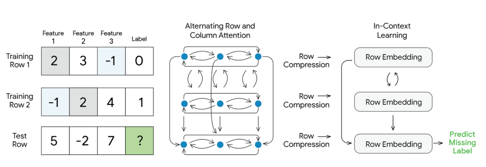
The diagram is honest about the shape and silent about the proportions. Three cells, three row embeddings, three boxes — nothing in it suggests that the right third of the picture is 1.62 billion parameters and the left two thirds are 19.5 million. It is also silent about the thirty-two members, about where categoricals are encoded, and about the fact that the left-hand table has already been through a scikit-learn pipeline before it arrives.
The zero-shot claim, mechanically
Here is what "a schema it has never seen" actually means. Nothing in the
1.64 billion parameters is indexed by column identity. No column-name
embedding. No per-schema head. No vocabulary. A column is a position, and the
only quantity the model knows about the schema is d, the count. That is why an
arbitrary table slots in: there is nothing to look up and fail to find.
The elegance has a price, and the price is that column order is now load-bearing
twice over. The cell embedder's three-way group is {h, h+1, h+3} mod d, so
moving one column rewrites every cell embedding in the table. And the row
attention puts RoPE on the column axis, so column position is a coordinate the
attention sees directly.
So the announcement's own framing — "tables are fundamentally two-dimensional and inherently orderless: swapping two rows or two columns does not change the underlying meaning" — is half true of TabFM. Rows are orderless in the model. Columns are not, and the default estimator spends 32 forward passes washing that out with random permutations.
Which brings us to a phrase worth reading carefully.
Trained on tables that do not exist
The pretraining story is one paragraph in the post and it is the most important paragraph in the release: TabFM is trained entirely on "hundreds of millions of synthetic datasets," generated on the fly from structural causal models with "a wide variety of random functions." No real tables. The stated reason is scarcity — big, diverse, licence-clean tabular corpora essentially do not exist, because the interesting tables are proprietary.
The generator is the evidence for that claim, so: here is the generator.
$ git -C tabfm ls-files 'tabfm/**/*.py' | grep -v _test
tabfm/src/__init__.py
tabfm/src/classifier_and_regressor.py
tabfm/src/hugging_face/convert_and_upload.py
tabfm/src/hugging_face/torch_convert.py
tabfm/src/jax/__init__.py
tabfm/src/jax/checkpointing.py
tabfm/src/jax/memory_efficient_attention.py
tabfm/src/jax/model.py
tabfm/src/jax/tabfm_v1_0_0.py
tabfm/src/pytorch/__init__.py
tabfm/src/pytorch/model.py
tabfm/src/pytorch/tabfm_v1_0_0.py
Twelve files, three of them __init__s: one scikit-learn wrapper, a JAX model
and a PyTorch model with their two config modules, a checkpoint loader, an
attention kernel, and two Hugging Face converters. No priors/, no data module,
no training loop, no sampler. The sentence that carries the entire release ships
without the code that would make it checkable.
This is the same bet TabPFN made in 2022 — and TabPFN shipped its prior, so at least the shape of the thing is on record. Its abstract promises one that "entails a large space of structural causal models with a preference for simple structures." In code that is a random MLP with noise at every layer, read rather than evaluated:
# automl/TabPFN at v1.0.0 (a9298ae), tabpfn/priors/mlp.py — get_batch()
def generate_module(layer_idx, out_dim):
    noise = GaussianNoise(...)  # one std per output dim, drawn once at init
    return [nn.Sequential(*[self.prior_mlp_activations(),
                            nn.Linear(self.prior_mlp_hidden_dim, out_dim), noise])]
...
outputs = [causes]
for layer in self.layers:
    outputs.append(layer(outputs[-1]))
outputs = outputs[2:]

if self.is_causal:
    ## Sample nodes from graph if model is causal
    outputs_flat = torch.cat(outputs, -1)
    random_perm = torch.randperm(outputs_flat.shape[-1] - 1, device=device)
    random_idx_y = list(range(-num_outputs, -0)) if self.y_is_effect else random_perm[0:num_outputs]
    random_idx = random_perm[num_outputs:num_outputs + num_features]
    y = outputs_flat[:, :, random_idx_y]
    x = outputs_flat[:, :, random_idx]
Read the last four lines. The columns of a synthetic table are not the inputs to a function; they are a random subset of the internals of one, and the label is another node from the same graph. That is what makes the dependence worth learning instead of trivial — the model never sees the causes, only a handful of downstream nodes, which is exactly the situation you are in with a real spreadsheet. Sample a few hundred million of those and a new table's dependence structure is recognisable in-context.
TabFM's generator is presumably bigger and better than this one. Nobody outside Google can say.
That bet has a second payoff the post does not claim, so I will claim it for
them: it forecloses benchmark contamination at the root. A model that never
saw a real table cannot have seen credit-g. Contrast this with Real-TabPFN, which
continues pretraining on curated real OpenML and Kaggle tables and consequently
has to build "an enhanced multi-tiered deduplication and filtering pipeline"
against every public benchmark to stay honest. TabArena itself is
contamination-aware — its leaderboard code carries a warning tag for entrants
that involve an LLM, reading "its results depend on a model whose training data
we cannot inspect and which may already have seen the test data." TabFM
correctly carries no such tag.
That is a real and underrated advantage, and I want it stated plainly before I come back, further down, to what it does not cover.
What the benchmark actually says
Both charts in the announcement are TabArena Elo. Here they are, reproduced from the post:
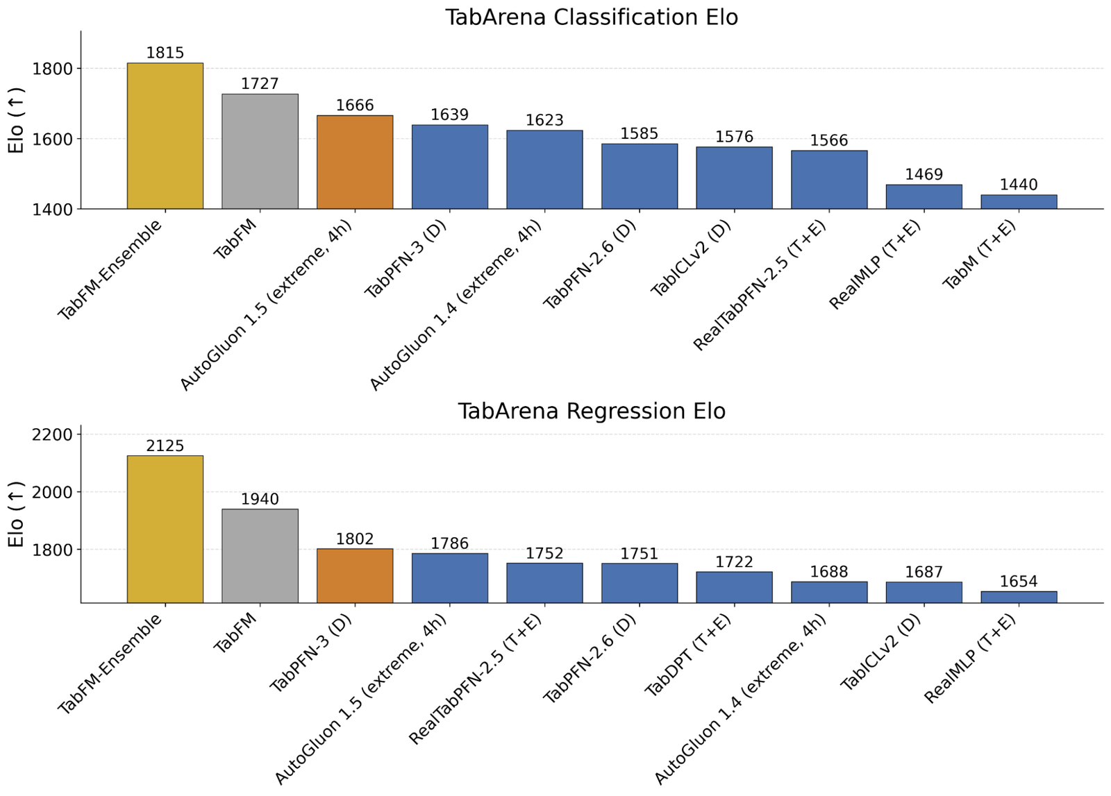
The post's opening paragraph names AdaBoost, XGBoost and random forests as the incumbents it is displacing. Not one gradient-boosted tree appears in either panel. Ten bars per chart, twenty bars total, zero trees. The nearest thing is AutoGluon, which is an AutoML system that stacks trees among other models. If you want to know where tuned CatBoost sits relative to TabFM you have to go to the leaderboard yourself.
So I did. Here is the live TabArena classification board on the day I wrote this, eleven weeks after release:
Two things fall out of that board that the announcement's chart does not.
The first is the actual gap to the incumbent. Tuned-and-ensembled LightGBM, the strongest tree on the board, sits 340 Elo below TabFM. On TabArena's scale — 400 points is a 91% expected win rate, and default random forest is pinned at exactly 1000 — that is a rout. It is also not a rout against a straw man: "tuned + ensembled" on TabArena means 200 randomly-sampled hyperparameter configurations per model, selected on an inner cross-validation and then post-hoc ensembled, with search spaces taken from the original papers or developed with the models' authors. The denominators hold up.
The second is that TabFM is now fifth. LimiX-2, TabPFN-3.5, TabPFN-3.5-Fast and Causilo have all landed since June. Nothing about the checkpoint changed.
Zero-shot TabFM beats tuned-and-ensembled CatBoost on 90.5% of TabArena folds. It loses to LimiX-2 on 67.5% of them. Same weights, same 51 datasets, same day — the number you quote is a choice of opponent.
| opponent | class | Elo | TabFM wins | fit s/1K | predict s/1K |
|---|---|---|---|---|---|
| LimiX-2 (default) | foundation model | 1973 | 32.5% | 30.94 | 9.028 |
| TabPFN-3.5 (default) | foundation model | 1890 | 48.5% | 1.84 | 0.473 |
| TabFM-Ensemble (TabFM+) | system | 1847 | 40.3% | 20.04 | 7.629 |
| AutoGluon 1.6 (noncommercial, 4h) | system | 1810 | 57.7% | 14.48 | 0.818 |
| TabFM (default) — the subject | foundation model | 1803 | — | 16.12 | 6.653 |
| AutoGluon 1.5 (extreme, 4h) | system | 1673 | 73.7% | 289.07 | 4.031 |
| TabPFN-3 (default) | foundation model | 1649 | 78.1% | 1.29 | 0.382 |
| TabPFN-2.6 (default) | foundation model | 1599 | 82.9% | 5.48 | 0.555 |
| TabICLv2 (default) | foundation model | 1583 | 84.8% | 0.75 | 0.139 |
| TabM (tuned + ensembled) | neural net | 1442 | 91.2% | 2450.13 | 2.247 |
| LightGBM (tuned + ensembled) | tree | 1426 | 90.7% | 417.05 | 2.639 |
| CatBoost (tuned + ensembled) | tree | 1416 | 90.5% | 1346.21 | 0.344 |
| XGBoost (tuned + ensembled) | tree | 1369 | 92.4% | 693.49 | 1.689 |
| CatBoost (default) | tree | 1376 | not published | 5.88 | 0.025 |
| RandomForest (tuned + ensembled) | tree | 1168 | 96.0% | 373.24 | 0.771 |
"Tuned + ensembled" on TabArena means 200 randomly sampled hyperparameter configurations per model, chosen on an inner cross-validation and then post-hoc ensembled, with the search spaces taken from the original papers or developed with the models' authors. These are not straw-man trees. Taking the same board's per-dataset mean errors and comparing pairwise rather than fold-by-fold, TabFM beats CatBoost (T+E) on 48 of the 51 datasets; it loses on hiva_agnostic, Amazon_employee_access and Diabetes130US. What the cost columns show is that the comparison is not like-for-like in the other direction either: CatBoost's 1,346 s/1K is search, paid once; TabFM's 16.1 s/1K is a forward pass over the context, paid on every call, and its 6.65 s/1K prediction is 19x CatBoost's.
The win rates are the number to quote, not the Elo, because Elo is not a property of the model at all.
The same TabFM weights carry at least six different TabArena Elo ratings, spread over 262 points, because Elo on a living leaderboard is a property of the pool and not of the model. Google's chart quotes the pair from the day of release.
| which pool | datasets | TabFM Elo | position | TabFM-Ensemble |
|---|---|---|---|---|
| Google's figure, classification, 30 Jun 2026 | 38 | 1727 | 2nd of the 10 shown | 1815 (1st) |
| Google's figure, regression, 30 Jun 2026 | 13 | 1940 | 2nd of the 10 shown | 2125 (1st) |
| live board, classification, models only | 38 | 1769 | 5th of 84 | not listed as a model |
| live board, classification, every entrant | 38 | 1777 | 5th of 86 | 1814 (3rd) |
| live board, regression, models only | 13 | 1989 | 4th of 83 | not listed as a model |
| live board, all 51 tasks, every entrant | 51 | 1803 | 7th of 86 | 1847 (3rd) |
TabArena's own code files TabFM-Ensemble (listed there as TabFM+) under method class 'System'; its constants.py comment reads "Whole pipelines rather than single models: AutoGluon, TabFM+, an agent, a hosted API." Google's chart plots it beside single models. Between release day and this capture LimiX-2, TabPFN-3.5, TabPFN-3.5-Fast, Causilo, EXAONE-Tabular and Mitra-v2 all entered the board; nothing about TabFM changed, and four entrants now sit above it on classification.
Same weights, six ratings, 262 points apart. The two Google plots are the two highest numbers available on the day of release. That is not dishonest — every one of these is a correct Elo for its pool — but "1815 versus 1666" reads as a fact about two models and it is a fact about a pool.
One more thing the chart flattens. TabArena's own code files TabFM-Ensemble
(which it lists as TabFM+) under method class System, with the comment
"Whole pipelines rather than single models: AutoGluon, TabFM+, an agent, a
hosted API." The announcement plots it beside single models, in the same chart,
as the top bar.
What the ensemble preset is actually buying
The TabFM-Ensemble configuration adds cross features, SVD features, a 32-way
non-negative-least-squares blend, and Platt scaling for binary problems. It is
worth 88 Elo on the release-day classification chart and 44 on the live
all-tasks board. Google committed the per-fold results for both configurations,
so this is checkable without running anything.
The preset itself is one classmethod, and the defaults it overrides are the whole story:
# tabfm/src/classifier_and_regressor.py — TabFMClassifier.ensemble()
@classmethod
def ensemble(cls, model: Any, **overrides: Any) -> "TabFMClassifier":
    params = dict(
        n_estimators=32,                         # unchanged — this is also the default
        average_logits=False,                    # default True: average probabilities instead
        n_feature_crosses="sqrt",                # default 0
        n_svd_features="sqrt",                   # default 0
        enable_nnls=True,                        # default False
        binary_calibration_method="platt",       # default None
        multiclass_calibration_method="vector",  # default None
    )
    params.update(overrides)
    return cls(model, **params)
Six flags, and n_estimators is not one of them — the preset does not add a
single forward pass to the thirty-two the default already runs. "sqrt"
resolves to max(1, int(np.sqrt(n_cols))) over the capped column count, so a
500-column member gets 22 crosses and 22 SVD directions. And it gets them on
half the ensemble, because the schedule is deliberately lopsided:
# the same file — EnsembleGenerator._get_member_n_features_list
k_max = self._get_n_features_to_add(n_features_requested, n_cols)
return [0 if i % 2 == 0 else k_max for i in range(self.n_estimators)]
Sixteen augmented views, sixteen plain ones, averaged together. A cross is a
product of two numeric columns (X[:, i] * X[:, j], categoricals excluded), and
the SVD is fitted on the full uncapped table before per-member subsampling —
which is why it rescues hiva_agnostic further down. The blend is non-negative
least squares on out-of-fold predictions, then pulled a quarter of the way back
to the uniform average by nnls_beta = 0.75. That is not nothing. It is also
not a second model.
The 44-Elo gap between TabFM and TabFM-Ensemble is worth a median of half a percent of error on the 30 binary tasks, and concentrates almost entirely in imbalanced and very wide tables. Computed from Google's own committed per-fold results.
| slice | datasets | folds | metric | ensemble wins folds | wins datasets | error cut |
|---|---|---|---|---|---|---|
| binary | 30 | 438 | ROC AUC | 59.4% | 21 / 30 | +0.50% |
| multiclass | 8 | 156 | log loss | 75.0% | 8 / 8 | +1.59% |
| regression | 13 | 222 | RMSE | 76.6% | 10 / 13 | +0.35% |
| all tasks | 51 | 816 | mixed | 67.0% | 39 / 51 | — |
| anneal — imbalance 85:1, 898 rows | 1 | 30 | log loss | — | — | +25.2% |
| APSFailure — 54:1, 170 features | 1 | 9 | ROC AUC | — | — | +25.1% |
| polish_companies_bankruptcy — 13:1 | 1 | 9 | ROC AUC | — | — | +17.3% |
| hiva_agnostic — 88:1, 1,617 features | 1 | 9 | log loss | — | — | +14.5% |
| churn — the worst single loss | 1 | 9 | ROC AUC | — | — | -2.23% |
TabArena scores binary tasks with ROC AUC. Platt scaling, which the ensemble preset adds for binary problems, is a monotone map and so cannot change ROC AUC at all — on 30 of the 51 datasets the calibration half of the preset is, by construction, invisible to the score. What is left is the feature crosses, the SVD features and the non-negative-least-squares blend, and their median return is half a percent. TabArena runs 10 repeats of 3-fold CV on datasets up to 2,400 rows and 3 repeats above 2,584, which is why the fold counts differ.
Across all 816 folds the ensemble preset wins 67.0% of them. But split it by task and the structure appears: on the 30 binary datasets — 438 folds, scored by ROC AUC — it wins 59.4% of folds, and the median dataset sees its error fall by half a percent. On the 8 multiclass datasets, scored by log loss, it wins 75.0% of folds and the median dataset improves 1.59%. On regression, 76.6% and 0.35%.
There is a mechanical reason the binary column is the weak one, and it is worth spelling out. Platt scaling is a monotone map. ROC AUC depends only on the ranking of the scores. On 30 of the 51 datasets, the calibration half of the "ensemble" preset cannot change the metric by construction. Log loss, which scores the multiclass tasks, is the one metric on TabArena that rewards calibration directly — and that is exactly where the preset earns its keep.
The rest of the gain is concentrated, not broad. The five biggest per-dataset
wins are anneal (+25.2%, class imbalance 85:1), APSFailure (+25.1%, 54:1,
170 features), polish_companies_bankruptcy (+17.3%, 13:1), hiva_agnostic
(+14.5%, 88:1, 1,617 features) and airfoil_self_noise (+12.6%). Four of the
five are imbalanced tables, and three of those are among the five TabArena flags
as extremely imbalanced. The honest summary of
TabFM-Ensemble is not "pushes performance further"; it is "recovers the
calibration and wide-table handling the base model lacks, on the minority of
datasets where that is what the metric is measuring."
Where it loses, and why
Taking the leaderboard's per-dataset mean test error, in each dataset's own metric, and comparing it pairwise against tuned-and-ensembled CatBoost: zero-shot TabFM wins 48 of 51. The three it loses:
| dataset | rows | features | imbalance | TabFM mean rank of 86 |
|---|---|---|---|---|
hiva_agnostic | 3,845 | 1,617 | 88:1 | 70.3 |
Amazon_employee_access | 32,769 | 9 | 16:1 | 34.8 |
Diabetes130US | 71,518 | 47 | 10:1 | 19.9 |
hiva_agnostic is the interesting one, because the mechanism is legible in the
code. max_num_features defaults to 500. With 1,617 columns, every one of the
32 ensemble members sees a random 31% slice of the table, and the three-way cell
group wraps modulo a different d in each. Mean rank 70.3 of 86 — TabFM's
worst result on the suite by a wide margin, worse than default XGBoost. Turn on
the ensemble preset, whose SVD features compress all 1,617 columns into dense
directions that survive subsampling, and it climbs to 21.6.
Amazon_employee_access is nine columns of high-cardinality identifiers. My
reading of TransformToNumerical is that a column arriving as pandas int64
takes the numeric path, which would Fourier-expand raw employee and resource
IDs as if they were continuous quantities — the failure mode CatBoost's ordered
target statistics exist to prevent. I have not verified the dtype TabArena hands
over, so that stays labelled as reasoning, with a falsifier below.
What does not show up is the degradation with dataset size that the "foundation models only win on small data" story predicts. Bucketing the 51 datasets by row count, TabFM's mean rank is 10.96 at ≤10k rows, 11.93 from 10k–100k, and 2.45 on the two datasets above 100k rows. Two datasets is not a trend, but it is not a collapse either.
Where contamination can still get in
Back to the claim above. Direct contamination is ruled out by construction: no real table went into pretraining, so no benchmark table did either. That is the strongest contamination posture any tabular foundation model can have, and it is stronger than the one belonging to every model on the board that fine-tunes on real corpora.
It is also unaudited. The repository contains inference code only. There is no prior, no generator, no training loop, and no report. "Hundreds of millions of synthetic datasets generated using structural causal models" is a sentence, and the property that sentence guarantees is the single load-bearing property of the release. Nobody outside Google can check it.
And there is a second channel, which synthetic pretraining does not close. A prior is designed. So is an architecture, and so are a dozen constants in the wrapper. Every one of those choices was made by people who could read TabArena, and three of them line up with it in ways worth noticing:
max_classes = 10, a hard architectural limit. The decoder's output dimension is 10. That is exactly TabPFN v2's ceiling, which TabArena's own paper cites as the constraint that limits where a tabular foundation model can be applied — so it is an inherited envelope, not an independent design. On the suite the ceiling is never within reach of binding: of the 8 multiclass tasks, six have exactly 3 classes, one has 5 and the hardest has 8.max_num_features = 500, the wrapper's default. Also TabPFN v2's number. Three TabArena datasets exceed it —Bioresponseat 1,776,hiva_agnosticat 1,617,QSAR-TID-11at 1,024 — and one of those three is TabFM's single worst result on the suite.- The dozen numbers nobody justifies.
softmax_temperature=0.9,outlier_threshold=4.0,nnls_beta=0.75,calibration_lambda=1e-2,min_rows_for_single_val_split=2000,num_folds_for_cv=5,norm_methods=["none", "power"],n_estimators=32. These are hyperparameters. They were tuned. "Eliminates the need for hyperparameter tuning" is a claim about your workload, not about the system, and the release does not say what corpus the defaults were fitted to.
None of this is evidence of anything improper. It is the difference between a contamination story that is structurally airtight and one that has actually been audited, and right now TabFM has the first and not the second.
One thing that is checkable, and that speaks well of TabArena: the board
re-runs entrants rather than taking submitted numbers. Google's committed
parquet results were produced with JAX on TPU; the leaderboard's TabFM row is
marked GPU and verified. Comparing the two on all 51 datasets, the median
absolute relative difference in mean test error is 0.23%, and 41 of 51 agree
within 1%. The exceptions are all datasets where the error is already tiny:
APSFailure (0.00739 on TPU against 0.00547 on the board — 35% relative, 0.0019
absolute), anneal (21.6%), polish_companies_bankruptcy (21.2%), and
hiva_agnostic, which is the only one with a material absolute gap (0.206
against 0.189). For a model whose compute dtype is bfloat16 and whose default is
a 32-member ensemble, that is about the reproducibility you should expect — and
it is a reason to read two-significant-figure wins on low-error datasets with
some suspicion, whoever is reporting them.
The limits, stated and unstated
The model card is unusually forthcoming, which I want to credit: it lists the 10-class ceiling as a "hard architectural limit", says memory scales with context rows, says behaviour on very wide tables "may degrade", and says outright that "performance on specific real-world domains, minority groups, or edge distributions is not fully characterised." That is a better limitations section than most releases get.
Here is what I would add to it.
The 10-class ceiling is never tested. The decoder's output dimension is literally 10; there is no way around it short of a new checkpoint. TabArena's hardest multiclass task has 8 classes and six of the eight have three. So the ceiling that defines the model's applicability is nowhere near exercised in the reported evaluation.
The README's own limits are wrong. The FAQ says the estimators expose
"max_num_features and max_num_rows (defaults are 500 features and 100
context rows)." The 500 is right. max_num_rows defaults to None in all three
places it appears — EnsembleGenerator, TabFMClassifier and TabFMRegressor
— meaning no cap, every training row goes into the context. Which is the more
important fact, because it is where the cost lives.
Regression is a separate model on a third of the evidence. There are two
checkpoints, not one. The regression stack swaps the Embedding[10, 256] label
lookup for an MLP[1 → 6 → 256] over the scalar target and the 10-way decoder
for a 1-way one, which is 1,647,783,213 parameters rather than 1,639,444,522 —
and arbitrary target scales are handled outside the model by a StandardScaler
on the training targets, inverse-transformed on the way out. TabArena's
regression slice is 13 datasets against classification's 38, and it is where
TabFM posts its highest Elo. Thirteen datasets is thin ground for the stronger
of the two headline numbers.
The cost profile inverts against trees. Median seconds per 1,000 samples on
TabArena: TabFM encodes its context in 16.1 and predicts in 6.65; tuned CatBoost
burns 1,346 to search and then predicts in 0.344. All in, that is 22.8 against
1,347 — 59× cheaper for a one-shot job you will never repeat. Against a tree
you have already fitted, it is 19× more expensive per prediction, forever,
and on a GPU rather than a CPU. And there is
no fitted artifact — there is a 6.25 GiB float32 checkpoint (12.5 GiB if you want
regression too) plus your entire training table, re-encoded on every call unless
you opt into cache_context=True.
The licence forbids the obvious use. The code is Apache-2.0. The weights are not.
So what changed
The honest answer to "why did tabular resist foundation models for so long" is that everyone was looking for the wrong shared substrate. There is no universal column vocabulary and there never will be. What TabFM — and TabPFN before it — found is that you do not need one: you need a model that has seen enough shapes of statistical dependence that a new table's dependence structure is recognisable in-context, and you get those shapes from a synthetic prior rather than from data.
What TabFM adds to that idea is scale, and the scale went somewhere specific. TabPFN v2's default classifier checkpoint is 27.7 MiB on the Hub and TabICL's is 103.3 MiB — if those are float32 weights, about 7.3M and 27M parameters. TabFM's is 6.25 GiB and 1,639,444,522 parameters, counted rather than inferred, with 98.8% of it in a transformer reading one token per row. The bet is that in-context learning over compressed rows is the part that benefits from depth, and the table-reading front end can stay tiny. On TabArena, in June, that bet paid: 1727 Elo against 1585 for TabPFN-2.6.
Eleven weeks later there are four models above it, and the two at the top — LimiX-2 at 1926 and TabPFN-3.5 at 1852 — get there at 36.96 and 1.85 median seconds per 1,000 samples against TabFM's 18.45. The category is moving fast enough that the interesting question is no longer whether a transformer can beat a tuned tree on a spreadsheet. It is which of these priors generalises to the table you actually have, and nobody — including Google, which has not released its generator — has published enough to answer that.
What would change my mind
7 claims above, and what would falsify each
TabFM's 'single forward pass' is thirty-two forward passes in the shipped default.
Read
TabFMClassifier.__init__intabfm/src/classifier_and_regressor.py:n_estimators: int = 32, withfeat_shuffle_method="random",class_shift=Trueandnorm_methodsdefaulting to["none", "power"]. If a future release drops the default to 1, or if someone shows the 32 members are fused into one batched call that is meaningfully "a single pass", this framing is wrong. I have measured the architecture, not the wall-clock.98.8% of TabFM's parameters are in a stage that never sees a cell.
Computed from the safetensors header of
google/tabfm-1.0.0-pytorch(classification/model.safetensors, 913 F32 tensors) by summing shape products per top-level module:icl_predictor= 1,619,925,002 of 1,639,444,522. Sum it yourself and get a different split, and the claim falls. The word "sees" is doing load-bearing work: the ICL stack reads 2048-d row vectors produced from cells, so it sees cells the way a language model's last layer sees characters.The binary half of TabArena cannot reward the ensemble preset's calibration step.
ROC AUC is invariant to any strictly monotone transform of the scores, and Platt scaling is one. If the preset's binary gain came from calibration rather than from crosses, SVD and NNLS blending, that would falsify it — the cleanest test is to run the preset with
binary_calibration_method=Noneand see whether the 30 binary datasets move at all. I have not run it; I inferred it from the metric and the code path.TabFM's weakness on Amazon_employee_access is high-cardinality categoricals taking the numeric path.
This is reasoning, not measurement.
TransformToNumerical.fitroutes any column wherepd.api.types.is_numeric_dtypeis true toSimpleImputer, not to the ordinal encoder, and nine integer-coded ID columns would qualify. Printclf.X_encoder_.tfm_.transformers_on that task's DataFrame as TabArena hands it over; if the columns land in thecategoricaltransformer, my explanation is wrong and the loss needs a different one. The loss itself is measured: mean error 0.14196 against CatBoost (T+E) at 0.11760.Synthetic-only pretraining forecloses direct benchmark contamination, but the claim is unverifiable as shipped.
The repository contains inference code only — no prior, no generator, no training loop. "Hundreds of millions of synthetic datasets from structural causal models" is a sentence in a blog post. Releasing the generator, or a technical report describing it, would settle this in either direction. Until then the correct posture is that TabFM's contamination story is structurally strong and evidentially unaudited — and that the wrapper's dozen tuned defaults (
softmax_temperature=0.9,outlier_threshold=4.0,nnls_beta=0.75,n_estimators=32) were fit to something nobody has named.Google's own TPU results and TabArena's verified GPU re-run differ by a median of 0.23%, and by up to 35% relative on the lowest-error datasets.
Merged the four parquet files in
google-research/tabfm/resultson(dataset, fold), averaged per dataset, and compared against theefield in the leaderboard's per-dataset payload forTabFM (default). 41 of 51 agree within 1%. I am attributing the gap to accelerator and backend — the parquet filenames sayjax-tpu, the board says GPU — and to bfloat16 compute over a 32-member ensemble. If the board's TabFM row turns out to be Google's own submitted numbers rather than a re-run, the comparison is between two things I have mislabelled and the inference is void.Elo on TabArena is a property of the pool, not the model.
Six ratings for one checkpoint, 1727 to 1989, captured 2026-09-19 from
website_leaderboard.csvacross entrant sets and task slices. If the ratings were stable across pools this would be a non-point. Re-pull the same files on a later date and the numbers will have moved again without a byte of the checkpoint changing — which is the claim, not a caveat about it.