The Skaling law: Chinchilla assumes model size and data don't interact, and they do

2026-08-10 · 12 min · scaling-laws · llm · math · training · explainer

The Chinchilla scaling law is one of the most quoted equations in the field. It says the loss of a language model decomposes into an irreducible floor plus two independent power-law terms, one for model size and one for training data:

L(N, D) = E + \frac{A}{N^{\alpha}} + \frac{B}{D^{\beta}}

Skaling: Chinchilla's Exponents Meet Kaplan's Coupling (arXiv 2608.07222, Mathurin Videau, Badr Youbi-Idrissi, David Lopez-Paz and Kartik Ahuja, FAIR at Meta, 7 August 2026) points at the plus sign in the middle and observes that it is a very strong claim nobody ever tested.

A sum of a function of $N$ and a function of $D$ has a cross-derivative of exactly zero. Not approximately zero, not small — zero, as an algebraic identity. The additive form asserts that how much a training token is worth does not depend on how big your model is. That assertion was never a finding. It was a modelling convenience that came along for the ride.

The saddle

Fit the additive law to a dense grid of trained models and the residuals are not noise. They have structure.

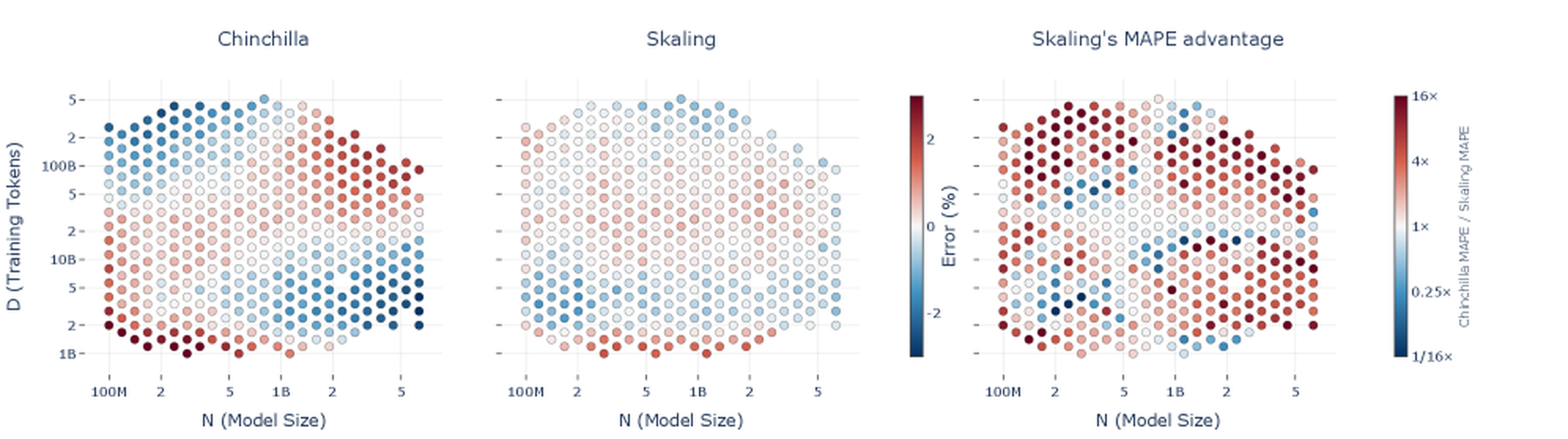
Three panels of hexagonally-packed markers over a grid of model size against training tokens. The Chinchilla panel shows a saddle pattern: strongly positive error in the bottom-left and top-right corners, negative in the top-left and bottom-right. The Skaling panel is much flatter and paler. The third panel shows Skaling's error advantage reaching sixteen-fold at the corners. — Signed percentage error of each fitted law across the (N, D) grid. Chinchilla is accurate in the interior and develops large, oppositely-signed errors toward the corners — the saddle shape you get when an N–D interaction is omitted (Videau et al., arXiv 2608.07222, Figure 1).

The paper's description of that first panel is precise: Chinchilla "is accurate in the interior of the grid but develops large, oppositely-signed errors toward the corners, reaching several percent where $N$ and $D$ are most imbalanced. This is the saddle-shaped residual expected when the $N$ – $D$ interaction is omitted."

A saddle is the signature of a missing product term. If your model of a surface has no $xy$ term and the true surface has one, the errors you get are positive on one diagonal and negative on the other — which is exactly what the left panel shows. The paper backs this up with a direct measurement of the cross-derivative $\partial^2 L/\partial N \partial D$ from local quadratic fits (their Figure 3), finding it non-zero and structured.

One exponent

The fix is small enough to state in a line. Kaplan's original 2020 form did couple $N$ and $D$ — $L(N,D) = [(N_c/N)^{\alpha_N/\alpha_D} + D_c/D]^{\alpha_D}$ — but it tied the inner exponents together through the ratio $\alpha_N/\alpha_D$ , so the per-axis decay rates were no longer independent. Chinchilla threw out the coupling to get the independence back. Skaling keeps both:

L(N, D) = \left(\frac{A}{N^{\alpha}} + \frac{B}{D^{\beta}}\right)^{k} + E

Chinchilla's interpretable base terms and independent inner exponents, raised to a single free outer exponent $k$ . At $k = 1$ it is the additive law — Chinchilla is a special case, not a rival. For any $k \neq 1$ the cross-derivative is non-zero. And because $k > 0$ , the loss is still strictly decreasing in both arguments, so adding capacity or data can never be predicted to hurt.

L(N,D) = (A/N^α + B/D^β)^k + EarXiv 2608.07222, Eq. 3

what one more token buys — |∂L/∂ln D| — at three model sizes10B benefits 1.62× as much as 100M

D = 1B tokensD = 10T tokens

N = 100MN = 1BN = 10B

k0.41

Set k = 1 and the three curves collapse onto one. That is the additive assumption stated in its most concrete form: how much a token is worth does not depend on how big your model is. Written as a derivative, ∂²L/∂N∂D = 0, exactly and by construction — not because anyone measured it, but because a sum of a function of N and a function of D cannot have a cross term. Slide k below 1 and the curves separate: bigger models get more out of the same token. The fitted value on this data is 0.41, which is a long way from 1.

The fitted value is what makes this more than a formality. On the Farseer grid, $k = 0.41 \pm 0.01$ — nowhere near 1, and tightly determined. Differentiating,

\frac{\partial^2 L}{\partial \ln N\, \partial \ln D} = k(k-1)\,\alpha\beta\left(\frac{A}{N^{\alpha}}\right)\left(\frac{B}{D^{\beta}}\right)R^{\,k-2}, \qquad R = \frac{A}{N^{\alpha}} + \frac{B}{D^{\beta}}

With $k < 1$ the factor $k(k-1)$ is negative, so the cross-derivative is negative: since $\partial L/\partial \ln D$ is already negative, making it more negative means bigger models extract more from the same token. That is not a surprising claim — it is roughly what everyone believes — but the additive law is structurally incapable of expressing it.

Interpolation quality is not evidence

This is the methodological point I most want people to take away, and it is stated bluntly in the paper: "High interpolation fit quality is not enough to validate a scaling law."

MAPE % · lower is better · Table 1

full grid5.0×10²² FLOPs

lawR²interpext Next Dfar

Chinchilla0.9950.771.481.982.46

Farseer0.9821.732.374.132.43

Skaling0.9980.410.470.882.31

sparse L-shape grid — low-compute edges only5.1×10²¹ FLOPs

lawR²interpext Next Dfar

Chinchilla0.9542.514.323.299.82

Farseer0.9741.812.072.522.37

Skaling0.9950.850.891.351.51

the headline comparison

Chinchilla, full grid
5.0×10²² FLOPsvsSkaling, L-shape
5.1×10²¹ FLOPs

1.48%ext N0.89%

1.98%ext D1.35%

2.46%far1.51%

Two things to read off this. First, the paper’s own warning: interpolation quality is not evidence. Chinchilla scores R² = 0.995 on the full Farseer grid and still extrapolates three to four times worse than Skaling. A law can fit the interior beautifully and still be wrong about how the surface bends outside it, which is the only thing you ever actually use a scaling law for. Second, the compute argument: Skaling fitted on the sparse L-shape grid — roughly a tenth of the FLOPs — extrapolates better than Chinchilla fitted on the whole thing, on every held-out regime.

Chinchilla achieves $R^2 = 0.995$ on the full Farseer grid. By the standard people usually apply, that is a solved problem. Its extrapolation error is three to four times Skaling's. The failure mode "is therefore not a poor fit to the interior, but a systematic misprediction of how the loss surface bends away from the observed region" — which is the only thing anyone ever uses a scaling law for. Nobody fits a scaling law to predict a run they already did.

The compute argument in the second half of that figure is the one with budget consequences. The authors pair the coupled form with an L-shaped sparse grid: instead of spreading held-out points across the whole $(N, D)$ plane, restrict training runs to the low-compute edges — a row of small models across many data budgets, and a column of small data budgets across many model sizes. Skaling fitted on that L-shape, at roughly a tenth of the FLOPs, extrapolates better than Chinchilla fitted on the entire grid in every held-out regime. On Farseer: 0.89% vs 1.48% on larger models, 1.35% vs 1.98% on more data, 1.51% vs 2.46% far outside both.

It is also worth reading the row that is not Skaling. The nine-parameter Farseer law is worse than three-parameter Chinchilla on several columns and carries huge fold-to-fold variance (±1.93 on far extrapolation). More parameters bought instability, not accuracy. The Skaling result is a one-parameter change that improves things, which is a different and much stronger kind of claim.

The part that changes decisions

Everything above is about fit quality. This is about where the money goes.

The compute-optimal token-to-parameter ratio $D^\star/N^\star$ is the quantity that answers "should the next dollar buy a bigger model or more data?" The paper recovers it two ways without assuming any parametric law — a global Gaussian-process surrogate and a local moving-least-squares surrogate, finding the point where the log-slopes balance — and then compares against what each fitted law predicts.

Two log-log panels of optimal tokens per parameter against training compute. Left: empirical optima from GP and MLS surrogates track the Skaling prediction downward while the Chinchilla prediction stays nearly flat. Right: power-law fits extrapolated to two times ten to the twenty-five FLOPs, where the empirical fits at slope minus 0.14 and minus 0.15 and Skaling at minus 0.11 fall steeply while Chinchilla at plus 0.03 rises. — Compute-optimal tokens per parameter, recovered without a parametric fit and compared against the analytic laws. The empirical exponents (−0.14, −0.15) are close to Skaling's (−0.11) and have the opposite sign from Chinchilla's (+0.03) (Videau et al., arXiv 2608.07222, Figure 6).

compute-optimal tokens per parameter · D*/N*exponents from Fig. 6

10¹⁸ FLOPs← observed data ends10²⁵

empirical (MLS)

m = -0.15

empirical (GP)

m = -0.14

Skaling

m = -0.11

Chinchilla

166

m = +0.03

compute10^24.0spread 4×

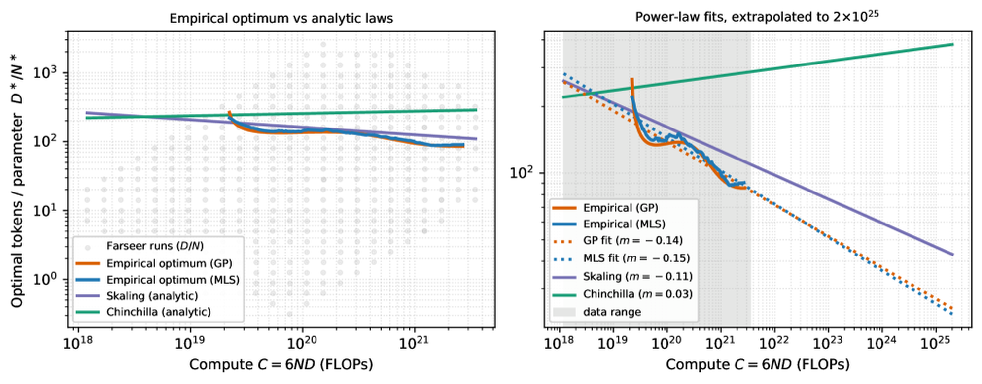
Inside the shaded region — where the runs actually are — all four agree, which is exactly why interpolation quality cannot tell you which law is right. Outside it they do not merely differ in magnitude, they differ in sign. The two model-free empirical estimates of the optimum slope downward at m ≈ −0.14; Skaling recovers −0.11; the additive law returns +0.03 and predicts you should train ever more overtrained models as compute grows. Extrapolate a few orders of magnitude and this is not an academic disagreement — it is the difference between spending a frontier budget on parameters or on tokens.

The two model-free estimates of the optimum give exponents of −0.14 and −0.15. Skaling recovers −0.11. The refitted additive law gives +0.03 — the opposite sign. Inside the observed data range all four agree, which is exactly why a good interpolation $R^2$ told you nothing. Outside it they diverge, and the paper reports that one order of magnitude beyond the data the allocations differ by more than 10×, with the additive law heading toward hundreds of tokens per parameter while the empirical fits and Skaling fall to the tens.

Two caveats before anyone reallocates a training budget on this. The empirical exponent is itself an extrapolation of a fit to a surrogate of a finite grid, and the two surrogates agreeing with each other is weaker evidence than two independent measurements. And "the additive law has the wrong sign" is a claim about these datasets, at these scales, with these architectures. But the sign disagreement is not subtle, it reproduces across two independently constructed grids, and it lands on the one number the whole scaling-law enterprise exists to produce.

What was actually measured

Worth being concrete about the evidence base, because scaling-law papers vary enormously here.

Farseer is an existing public grid; the fitting set is 302 configurations totalling ~5.0×10²² FLOPs, with held-out sets for larger models (36 points, 1.5B–6.4B), more data (66 points), and far extrapolation (7 runs at 2.3B–25B parameters on 126B–453B tokens, beyond both axes). SK-Grid is the authors' own: 134 configurations, 15 model sizes from 134M to 4.9B, 16 data budgets from 316M to 316B tokens, with far-extrapolation runs at ~10²² FLOPs on 5.8B–10.8B parameter models. Two more datasets appear in the appendix with the same protocol and the same ranking.

All laws are fitted identically — Huber loss in log space, L-BFGS-B with 2000 basin-hopping restarts, analytic gradients — so the comparison is not confounded by one law getting a better optimizer. The paper also notes that the improvement survives holding the protocol fixed, "confirming the gain comes from the functional form rather than the protocol."

What is not here: no runs at frontier scale, so the far-extrapolation column tops out around 25B parameters; no test of whether $k$ is stable across architecture families, tokenizers or data mixtures, which is the obvious next question given that $k$ is now carrying the entire interaction; and no mixture-of-experts models, where "model size" is ambiguous enough that it is unclear which $N$ even belongs in the formula.

Redoing my own arithmetic

Four days ago, writing about liquid time constants and gated delta rules, I used the additive Chinchilla form to estimate a confound. The setup: a 29M-parameter model, LTCAttention, beat its baseline by 0.062 nats on a token-matched comparison while running 12.4% slower. I asked what the baseline would have gained if it had spent that 12.4% on extra tokens instead, got roughly 0.061 nats, and concluded that a compute-matched comparison might erase the entire result.

I used Hoffmann et al.'s 2022 coefficients. This paper supplies two better options: the same additive form refitted on Farseer, and the coupled form on the same runs.

the same back-of-envelope under three lawsN = 28.8M · D = 287.6M · D/N = 10

lawpredicted gain from more tokenstokensparams

Chinchilla · Hoffmann 2022

the coefficients I used originally

0.06100.0048

Chinchilla · refit on Farseer

same functional form, this paper's fit

0.03050.0015

Skaling · fit on Farseer

coupled form, same runs

0.02560.0008

measured LTC effect

0.0619—

+1.2% params+12.4% tokens

At the defaults — LTCAttention’s actual +1.20% parameters and its 12.40% throughput penalty spent on extra tokens instead — the three laws span 2.4×. Most of that gap is not the coupling at all; it is that Hoffmann’s 2022 coefficients were fitted on a different corpus and tokenizer, and refitting the same additive form on Farseer halves the answer. The coupled form then trims it further. The number I published was the most pessimistic corner of that range, and this configuration sits at D/N = 10 — inside the band where the paper reports the additive law is at its worst.

The three answers span 2.4×. The estimate I published was the largest of them.

Most of the movement is not the coupling — it is that Hoffmann's coefficients were fitted on a different corpus and tokenizer, and refitting the same functional form on Farseer roughly halves the answer, from 0.061 to 0.031 nats. The coupled form then trims it further, to 0.026. There is also a pointed detail: LTCAttention's configuration sits at $D/N = 10.0$ , which falls in the band the paper reports as Chinchilla's worst regime — 3.47% MAPE in the optimal-ratio third, where its pooled number hides the failure.

So the honest revision: a compute-matched baseline would probably have recovered somewhere around half of LTCAttention's measured gain, not all of it. The conclusion I actually drew still stands — the missing experiment is a wall-clock-matched run, and until someone does it the result is better per token and undetermined per second — but I stated the confound about twice as strongly as the evidence supports. That correction is now in the record here rather than only in my own notes.

The broader lesson is the one I would take from this paper even if I had no stake in it. Scaling-law arithmetic is routinely used the way I used it: pull the canonical coefficients, differentiate, get a number, cite it as though it were a measurement. It is not. It is a prediction from a functional form fitted to somebody else's grid, and both the form and the grid are doing real work. When the answer matters, quote the range.

The take

The contribution is one exponent, and the reason it is a good paper rather than a small one is that the exponent is load-bearing. It removes a structural bias that was invisible in interpolation error and severe at the boundaries, it makes accurate extrapolation possible from a tenth of the compute, and it flips the sign of the trend in the single number the field uses to allocate training budgets.

What it does not do is settle anything at frontier scale, where nobody has published the grid that would test it. And there is a mild irony worth naming: the paper's own argument implies that its $k = 0.41$ is a property of these datasets, and the honest way to use the Skaling law is to refit it on your own runs rather than to quote 0.41 the way people have been quoting 20 tokens per parameter for four years.

Sources: Skaling: Chinchilla's Exponents Meet Kaplan's Coupling (arXiv 2608.07222v1, Videau, Youbi-Idrissi, Lopez-Paz, Ahuja, FAIR at Meta, 7 August 2026, CC BY 4.0), read in full via the arXiv HTML rendering. Equation 3, the fitted coefficients in Table 2, the MAPE figures in Tables 1 and 3, and the compute-optimal exponents in Figure 6 are quoted as published. Both figures are the paper's own, flattened onto white. The cross-derivative expression, the recomputation of my earlier LTCAttention estimate, and the sensitivity arithmetic behind the last interactive are mine, computed from the paper's published coefficients at LTCAttention's reported N and D. All four interactives are mine.