Reading a torch.profiler trace: overhead-bound vs compute-bound

Every "my GPU is slow" bug is one of two things: the GPU is doing too much work, or it is doing nothing while the CPU flails. You cannot tell which by staring at the code. You attach a profiler and read the trace. Hugging Face's torch.profiler guide teaches this with the smallest possible workload — y = matmul(x, w) + b, bf16, on an NVIDIA A100-SXM4-80GB — and shows the same three lines of code land on opposite ends of that spectrum depending only on the matrix size. This is a walk through what the profiler prints, how to read it, and the two bottleneck regimes it exposes.

The 20-line setup

The workload is deliberately trivial so the profiler output is the whole story, not the model:

# 01_matmul_add.py — profile y = matmul(x, w) + b on an A100, bf16
import torch
 
N = 64  # start small; bump to 4096 later
x = torch.randn(N, N, dtype=torch.bfloat16, device="cuda")
w = torch.randn(N, N, dtype=torch.bfloat16, device="cuda")
b = torch.randn(N, N, dtype=torch.bfloat16, device="cuda")
 
def fn(x, w, b):
    return torch.add(torch.matmul(x, w), b)
 
def step():
    with torch.profiler.record_function("matmul_add"):   # a named region in the trace
        fn(x, w, b)

record_function("matmul_add") is the one line people skip and then regret: it draws a labelled box around your code in the trace so you can find it among thousands of aten::* ops. The harness wraps step() in the profiler:

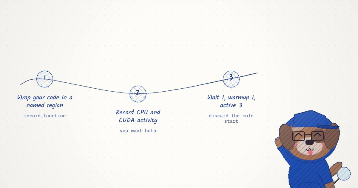
schedule = torch.profiler.schedule(wait=1, warmup=1, active=3, repeat=1)
 
with torch.profiler.profile(
    activities=[
        torch.profiler.ProfilerActivity.CPU,
        torch.profiler.ProfilerActivity.CUDA,
    ],
    schedule=schedule,
) as prof:
    for _ in range(5):          # 1 wait + 1 warmup + 3 active = 5 steps
        step()
        prof.step()             # advance the schedule one step
 
print(prof.key_averages().table(sort_by="cuda_time_total", row_limit=15))
prof.export_chrome_trace("trace.json")   # open in https://ui.perfetto.dev

Two knobs matter here. activities records both CPU-side dispatch and CUDA kernels — you want both, because the whole point is comparing them. schedule decides which steps count.

schedule: which steps land in the trace

prof.step() advances a little state machine. wait steps are skipped entirely, warmup steps run but get discarded, active steps run and get recorded. The warmup exists to throw away the first-step cold start — on step zero the CPU sits idle for a couple hundred microseconds before it issues its first launch, and you do not want that artifact averaged into your numbers.

With wait=1, warmup=1, active=3 over range(5), exactly 3 steps are recorded — which is why every row in the table below reads # of Calls = 3, and why the first recorded box in the trace is labelled ProfilerStep#2.

Reading the table: Self CPU vs Self CUDA

key_averages().table() is the first thing to read, before any timeline. Here is the 64x64 run, sorted by CUDA time:

expand

The two columns that decide everything are Self CPU and Self CUDA. Self time is a row's own time, excluding its children — so aten::matmul shows big CPU total but ~0 self time (its work lives in the child aten::mm and the kernel it launches). Read the self columns and the picture is stark:

• Self CUDA time total: 23.104 us. The GPU does 23 microseconds of real work. That splits into two kernels — the GEMM (ampere_bf16_s16816gemm_bf16_64x64_..., 14.272 us, ~62%) and a vectorized_elementwise_kernel for the add (8.832 us, ~38%).
• Self CPU time total: 2.314 ms — a hundred times larger. And 1.786 ms of it (77.20%) is a single row: cudaDeviceSynchronize, the CPU blocking to wait for the GPU.

When Self CPU dwarfs Self CUDA like this, the GPU is starved. The kernel isn't slow; there is barely any kernel. This is overhead-bound.

Reading the trace: two lanes, one dependency

The table tells you what is expensive; the timeline tells you when and why there are gaps. Export the trace, open it in Perfetto, and you get two lanes that matter — the CPU main thread and the GPU stream:

expand

The mental model: the CPU launches, the GPU executes, and the two lanes are offset in time. The CPU calls cudaLaunchKernel, which returns almost immediately — the kernel is queued, not run. The GPU picks it up a moment later on its own stream. So a fast CPU op and a slow GPU kernel show up as staggered boxes, not stacked ones. The dashed dependency in the diagram below is that hand-off.

In the 64x64 trace the GPU lane is nearly empty: 23 us of kernels scattered in a wall that is milliseconds wide. The GPU is idle roughly 98% of the time. Flip the interactive to see the same lanes fill up when the matrices grow:

Same code, two regimes

Change one number — N = 64 to N = 4096 — and rerun. Nothing else moves. The table inverts:

At 4096, Self CUDA (4.495 ms) finally rivals Self CPU (4.908 ms). One kernel — ampere_bf16_s16816gemm_bf16_128x256_..., 4.285 ms, 95.33% of GPU time — is now the entire budget. Note the tile even changed: cuBLAS picks a 128x256 GEMM tile for the big matrices where it used 64x64 for the small ones. cudaDeviceSynchronize is still 94% of the CPU wall, but the reading is different: here the CPU is legitimately blocked on real GPU work, not spinning on launch overhead. Same row, opposite meaning — which is exactly why you read both lanes.

The verdict changes what you do next:

• Overhead-bound (64x64): stop launching so many tiny kernels. Batch more work per launch, fuse ops, or hand it to torch.compile. Making the kernel faster buys you nothing — it is already 23 us.
• Compute-bound (4096x4096): the gemm is the job. Optimize the kernel — lower precision, better tiling, a fused epilogue — or reduce FLOPs. Cutting launch overhead buys you nothing here.

What torch.compile actually does here

The obvious fix for the overhead-bound case is to stop dispatching matmul and add as two separate ops. torch.compile does that:

cfn = torch.compile(fn)
 
def step():
    with torch.profiler.record_function("matmul_add"):
        cfn(x, w, b)

In the trace, the two ops collapse into a single aten::addmm dispatch — a GEMM with the bias folded into its epilogue instead of a separate elementwise kernel:

expand

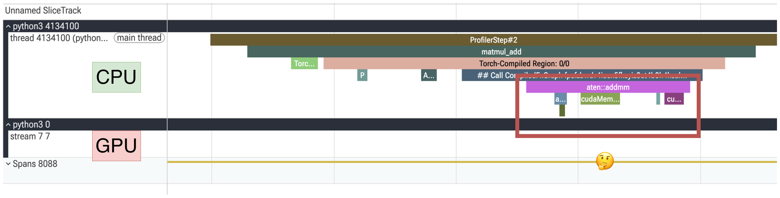
Two things are worth seeing honestly. First, there is still a Device-to-Device cudaMemcpyAsync in the region — the bias has to be staged/broadcast before it folds into the GEMM, so "fused" does not mean "zero extra work". Second, the compiled path adds its own CPU cost: a CompiledFxGraph call plus Dynamo's guard and cache lookup roughly double the per-step CPU overhead versus eager. Underneath, it is still the same ampere cuBLAS GEMM kernel doing the math.

So torch.compile is a real win when the fusion removes launches across many ops or feeds a big epilogue — but on a single matmul + add over small inputs, its fixed dispatch overhead is not amortized and can cost more CPU than it saves. The profiler is how you tell the difference instead of guessing. Measure both, keep the faster one.

The workflow, condensed

• Wrap regions with record_function("name") so you can find your code in the trace.
• Use a schedule with at least one warmup step; discard the cold start.
• Read key_averages().table() first. Compare Self CUDA total vs Self CPU total to get the regime.
• Then open the trace in Perfetto. CPU lane launches, GPU lane executes, offset in time. Empty GPU lane = overhead-bound; a fat kernel filling the GPU lane = compute-bound.
• Fix the regime you actually have. Fuse/batch for overhead; optimize the kernel for compute. Re-profile to confirm the win is real and not a torch.compile tax.

None of this needs a big model. A 64x64 matmul on an A100 is enough to show the difference between a GPU that is busy and a GPU that is waiting — and that difference is most of GPU performance work.

Built on Hugging Face's Understanding the torch.profiler (2026). All timings are the post's A100 / bf16 runs, reproduced from its key_averages() tables and Perfetto traces for commentary; the TraceLanes and ScheduleStrip widgets are redrawn illustrations of the mechanism, not live captures.