EVA: a VAE that samples well once its prior predicts the next latent

mdjsonmcpcopy↗ai

2026-10-06 · 21 min · vae · autoregressive · image-generation · audio · diffusion

Why read this

Notable· top 60%

Why one Gaussian per step suffices in a learned latent, EVA's prior heads counted in the weights, and three paper-vs-release mismatches.

• Original analysis
• Runs on a consumer GPU
• A lasting reference

·Image & video generation·MIT·Research paper

How this was scored

Is it new?

2 of 3: A real new idea, method or capability

Can I trust it?

2 of 3: Measures key facts from files, code or configs

Can I run it?

2 of 3: Open code or weights with real limits

Will I understand it?

2 of 3: Mechanism from first principles with figures

Can I act on it?

2 of 3: A concrete recipe, numbers or comparison

Will it last?

2 of 3: A reference for a year or more

Does it affect many?

1 of 3: A specialist community

Only here?

2 of 3: A teardown or measurement few others did

Score 66 of 100, ranked 157 of 445 rated articles. Each question is answered 0–3 by hand, and a 3 is rare. How articles are scored

Kaede Shiohara's announcement made a claim I didn't believe on first read. It said VAEs could be revived for sequential generation "only with an extra single linear layer that predicts the next prior without VQVAEs or diffusion models". For about five years, VAEs in image generation have been the compressor, not the generator. Stable Diffusion's KL-f8, MAR's KL-16 and DC-AE all encode pixels into a latent, and then something heavier (a diffusion model, a flow, a masked transformer) learns to produce that latent. Nobody samples from the VAE's own prior, because the pictures that come out of it are mush.

So the claim that one linear layer fixes this sent me to the paper (arXiv 2610.06545), the project page and the code. I expected some clever prior, perhaps a flow or a learned mixture. The new weights turned out to be two nn.Linear(768, 128). The interesting part is not the layer. It is what the layer lets the rest of the network stop doing.

expand

Why you can't sample from a VAE

A VAE trains two networks against one bound. An encoder $q_\phi(\mathbf z\mid\mathbf x)$ maps data to a Gaussian over latents. A decoder $p_\theta(\mathbf x\mid\mathbf z)$ maps latents back. Both are fitted by maximising the evidence lower bound:

The prior $p(\mathbf z)$ is almost always $\mathcal N(\mathbf 0,\mathbf I)$. At generation time you draw $\mathbf z$ from that prior and decode. This only works if the latents the encoder actually produces, pooled over the whole dataset (the aggregate posterior), look like the prior. In practice they don't. The reconstruction term pulls each image's latent toward wherever it decodes best. The KL term pulls it back toward the origin. The compromise leaves regions the prior assigns real probability that no training image ever occupied, the "prior holes". Draw from one of those and the decoder has never been taught what to do.

For a single global latent, as in the classic MNIST VAE, that is the whole story. EVA works on a sequence: a 16x16 grid of tokens for an image, 215 tokens for nine seconds of audio. Here there is a sharper version of the problem, and it is the one the paper is really about. With a factorised prior, the KL is paid per token. Each token's latent can match $\mathcal N(0,1)$ perfectly on its own, while neighbouring tokens stay strongly dependent on each other. The prior then samples every token independently, so the joint it hands the decoder has the right marginals and the wrong structure. A patch of sky is drawn without knowing that the patch above it was sky.

The widget below shows that failure on two neighbouring tokens. The blue cloud is a correlated Gaussian whose marginals are exactly standard normal, so a per-token KL to $\mathcal N(0,1)$ has nothing left to complain about. The orange cloud is what the prior draws.

At $\rho = 0.85$, 332 of 900 independent draws (36.9%) land outside the region holding 95% of the real latents; chance would put 47 there. Push the correlation to 0.95 and it is 539 of 900. The gap has a closed form. The KL between a correlated joint and the product of its marginals is the mutual information, $-\tfrac12\log(1-\rho^2)$: 0.641 nats per pair at 0.85. No per-token standard-normal prior can pay that down, however well each token is regularised. Switch the prior to "autoregressive" and the second token is drawn from $\mathcal N(\rho z_t,\,1-\rho^2)$, its true conditional. The off-region count falls back to 47, which is chance.

The widget is a toy I built, not the paper's data. The paper does show the real version, though. In its latent visualisation (Figure 4, further down) the causal VAE's posteriors "still exhibit a few spatially structured variations" despite the KL pressure. That is exactly the dependency the factorised prior throws away.

The one change: a prior that reads the past

EVA keeps the ELBO and changes the factorisation. Write the data and latents as sequences of length $T$, $\mathbf x = x_{1:T}$ and $\mathbf z = z_{1:T}$. Then assume three things (paper, Eqs. 12-14): a causal decoder, an autoregressive prior, and a mean-field posterior.

Substitute them into the ELBO. Because the decoder only looks backwards and the prior is a chain, the bound splits into one term per position (Eq. 15):

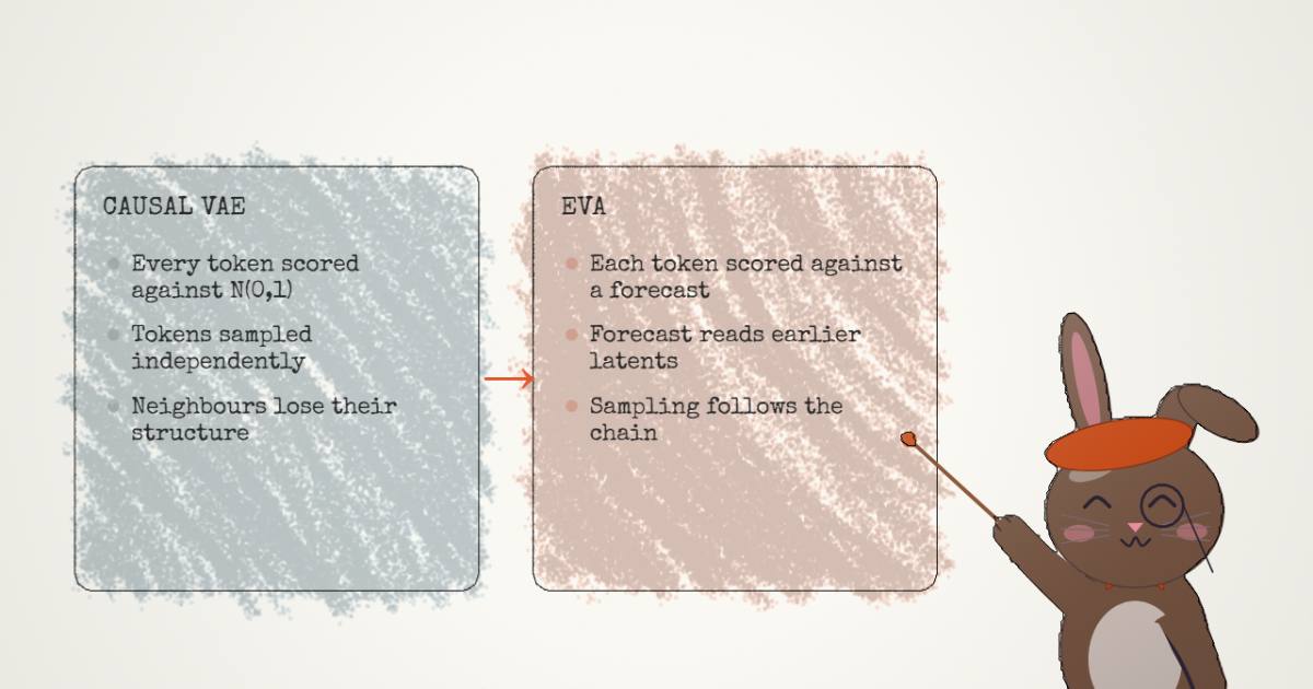
Read the KL term slowly, because it carries the whole method. The posterior for token $t$ sees the entire input $\mathbf x$, since the encoder is a full-attention transformer. The prior for token $t$ sees only the sampled latents before it. Training pushes the prior's guess toward where the encoder actually put $z_t$, given what came before. Where a standard VAE scores every token against the same fixed target, EVA scores each one against a forecast.

The forecast is a diagonal Gaussian, $p_\omega(z_t\mid z_{1:t-1})=\mathcal N(z_t;\hat\mu_t,\hat\sigma_t^2)$, with $\hat\mu_t$ and $\hat\sigma_t$ read off the previous latents (Eq. 16). The KL between two diagonal Gaussians has a closed form, so the loss needs no sampling beyond the usual reparameterisation:

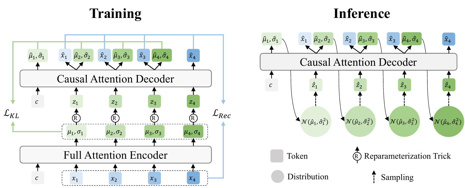
Sampling is ancestral. Draw $z_1$ from the first prior, decode $x_1$, feed $z_1$ back to get the prior for $z_2$, and so on for every position. It is an autoregressive model, but over a latent that the model designed for itself.

expand

Where the linear layer actually lives

"An extra single linear layer" is accurate, but only next to the right baseline. The paper's baseline is a causal VAE: the same full-attention encoder, a 12-block causal transformer decoder, and a standard-normal prior. EVA adds one thing to that baseline. The decoder's hidden state at position $t$ already exists to reconstruct $x_t$, and now it also forecasts $z_{t+1}$. In models/eva.py that is two heads next to the reconstruction head:

self.output_head = nn.Linear(transformer_latent_dim, self.token_embed_dim)
 
self.decoder_prior_mu = nn.Linear(transformer_latent_dim, reparam_dim)
self.decoder_prior_logvar = nn.Linear(transformer_latent_dim, reparam_dim)

I read the safetensors header of the released mapooon/eva-imagenet-base-128-ema checkpoint without downloading the weights. Those two heads hold 196,864 parameters out of 171,405,072, which is 0.11%. The paper's Table 1 lists EVA at 171.8M for training and 86.4M for inference. From the file I get 171.4M and 86.1M (decoder, prior heads, embeddings). That is close, but I can't reproduce the paper's decimals.

The bookkeeping that lines the forecasts up with the right targets is the part worth reading. The prefix is four register tokens and a class token. The class token's hidden state forecasts the first latent. Every image position then forecasts the one after it, and the last forecast is dropped:

# Raw image-position priors: index t predicts next latent z_{t+1}.
mu_img = self.decoder_prior_mu(hidden)
logvar_img = self.decoder_prior_logvar(hidden).clamp(-10.0, 10.0)
# class token is treated as z_{-1}; its prior predicts z_0.
class_idx = self.register_token_size
class_hidden = hidden_full[:, class_idx:class_idx + 1, :]
mu_class = self.decoder_prior_mu(class_hidden)
logvar_class = self.decoder_prior_logvar(class_hidden).clamp(-10.0, 10.0)
# Align to q(z_t): [z_0 from class] + [z_1.. from image 0..T-2]
mu_aligned = torch.cat([mu_class, mu_img[:, :-1, :]], dim=1)

The loss is the two terms added with no weight between them: total_loss = recon_loss + kl_loss (models/eva.py:484-486), where the first is F.mse_loss on the tokenizer latents and the second is the closed-form KL above. There is no stop-gradient anywhere. The KL pulls the prior toward the posterior and, just as hard, pulls the posterior toward the prior. That symmetry matters, and the next section is about why.

Put plainly, the 12-block causal decoder already was an autoregressive transformer over latents. The linear heads turn its spare capacity into a density, and the KL makes the encoder put latents where that density can find them. The decoder does double duty, so at inference EVA-B runs 86M parameters. The AR baselines in the paper run all 171M at inference for the same training budget, because without an encoder to discard, all 24 blocks are on the generation path.

Why one Gaussian per step is enough

This is the part that made me take the paper seriously.

Continuous autoregressive image models all hit the same wall: the next token is multimodal. The patch after a dog's ear could be more ear, background or a collar. The field's answers make the per-token head more expressive. GIVT puts a Gaussian mixture on top of the transformer. MAR puts a small diffusion model there and pays for it with tens of denoising steps per token.

EVA's forecast is a single diagonal Gaussian, the least expressive head you could pick. It can still produce multimodal images because of where that Gaussian lives. It is not a distribution over pixels or over tokenizer latents. It is a distribution over $z$, a space the encoder is free to shape, and between $z$ and the output sits a nonlinear decoder. The paper's Section 3.3 says this precisely (Eq. 26). Marginalising a Gaussian decoder over a continuous latent gives a continuous mixture of Gaussians, which can have as many modes as it needs. The decoder bends one bell curve into several.

The widget makes that concrete. It uses the observation spacing of the paper's toy (modes 2.4 apart, width 0.05, Appendix B.1). Each row is a hand-built version of a model family, not a trained network.

With four target modes, a mean-squared-error regressor puts all its mass at the mean, which is between modes by construction. A three-component mixture has to cover four modes with three bumps, and in my construction 37.1% of its mass ends up between modes. The latent route makes any number of modes from one Gaussian. What it leaks depends on how sharply the decoder can step: 25.6% at sharpness 15, 12.8% at 30, 6.4% at 60. It never quite reaches zero. A smooth decoder cannot place zero density between two modes it reaches continuously.

That is also what the paper's own toy shows, and it is the figure I'd point anyone to first.

expand

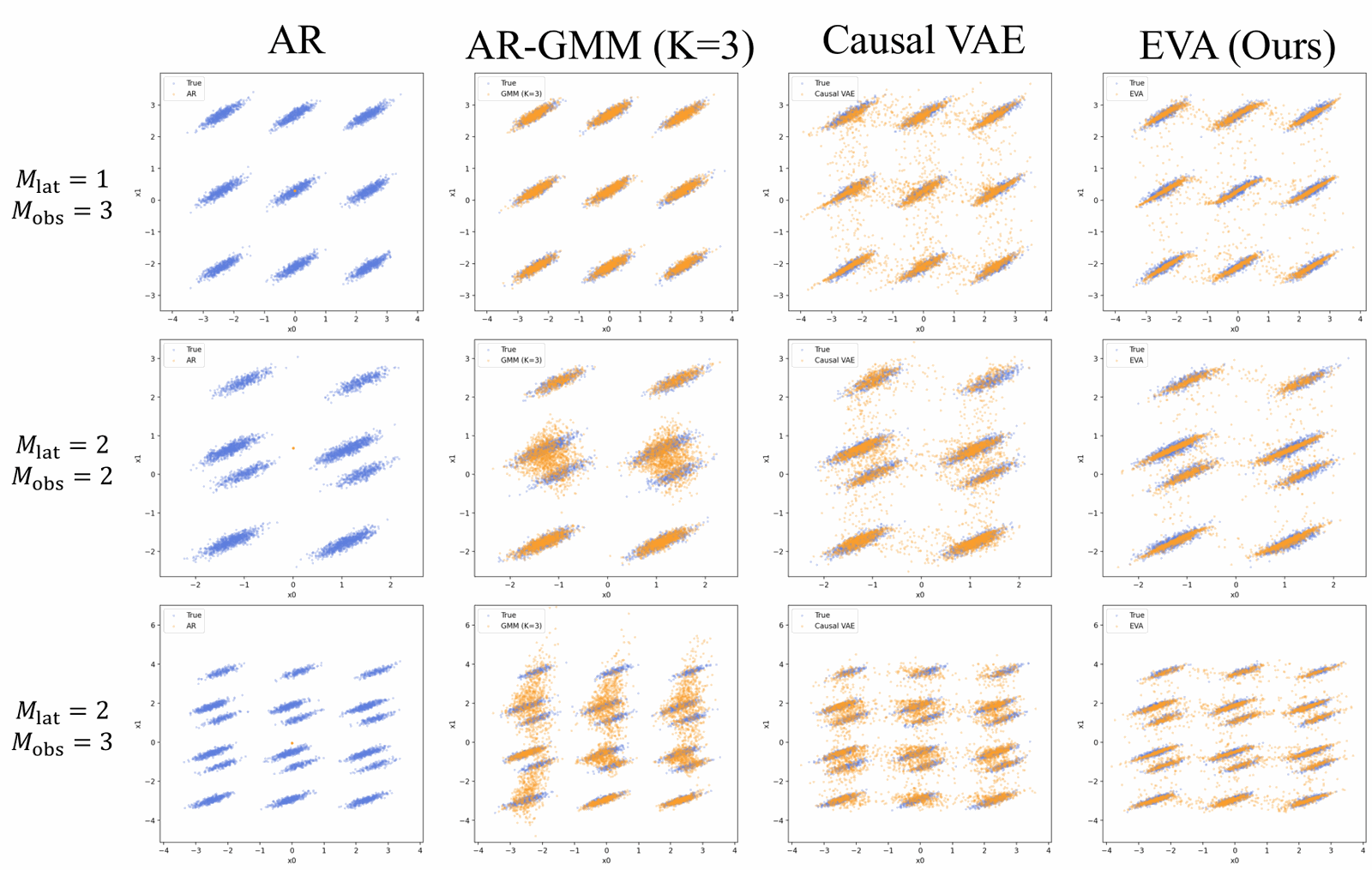
The causal VAE column is the interesting comparison. It has the same continuous-mixture decoder, so it finds every cluster. What it lacks is a prior that knows which cluster the first step chose, so the second step is drawn as if the first had never happened. That produces the orange spray between clusters, the same independence failure as the corners of the widget at the top of this page.

The symmetric KL is why all this works. Because the posterior is also pulled toward the forecast, the encoder learns to put $z_t$ where a Gaussian centred on a function of $z_{1:t-1}$ would expect it. Multimodality has to be expressed somewhere. EVA pushes it out of the latent transition and into the decoder's bend. Diffusion heads take the opposite trade: a simple space and an expensive head. EVA takes a learned space and a cheap head.

Sampling, and a guidance schedule the paper leaves out

Generation is a KV-cached loop over 256 positions for an ImageNet image. Each step is one 12-block decoder forward on one token, a draw from the forecast Gaussian, and a deterministic read-out of the next tokenizer latent. The read-out adds no noise: next_token = preds (models/eva.py:570). Every bit of randomness in an EVA image comes from the $z$ draws.

Classifier-free guidance acts on the forecast mean. The paper gives it as Eq. 27 with a fixed $s = 7$:

The code does something slightly different, and it changes how to read "CFG 7":

@staticmethod
def _guidance_scale_for_step(step, total_steps, guidance_scale):
    return 1.0 + (guidance_scale - 1.0) * float(step + 1) / float(total_steps)
 
@staticmethod
def _guided_prior_params(mu_cond, logvar_cond, mu_uncond, logvar_uncond, scale):
    mu = mu_uncond + scale * (mu_cond - mu_uncond)
    alpha = float(max(0.0, min(1.0, scale)))
    precision = (1.0 - alpha) * torch.exp(-logvar_uncond) + alpha * torch.exp(-logvar_cond)

The scale ramps linearly over the sequence. The first token is guided at about 1.02 and only the last token gets the full 7; averaged over 256 positions the scale is about 4.0. The variance is a precision blend. For any scale of 1 or more, alpha clamps to 1 and the conditional variance is used unchanged. Neither choice is wrong. MAR uses a similar linear CFG ramp, and EVA's repository is built on MAR's codebase. But anyone reproducing Table 1 from the paper text alone would use a constant 7 and get different numbers. The released ImageNet generation configs set guidance_scale: 7.0, and VGGSound's uses 10.0.

The numbers, and the comparison they're in

Every model in Table 1 shares one 170M training budget: 24 blocks at width 768. EVA and the causal VAE split it into a 12-block encoder and a 12-block decoder. The AR baselines use all 24 for a causal transformer. All of them were trained 400 epochs on the same KL-16 tokenizer latents.

expand

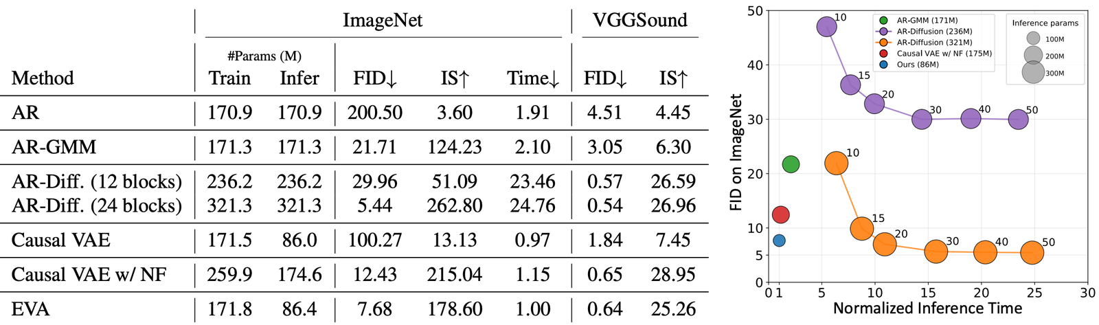
The ablation is the cleanest thing in the table. Going from the causal VAE to EVA adds only the linear heads and the prior they make possible, and ImageNet FID falls from 100.27 to 7.68 while IS climbs from 13.13 to 178.60, at essentially the same inference time (0.97 against 1.00). A normalising-flow prior in the SimFlow style also rescues the causal VAE, to 12.43, but it adds 88.1M parameters to do it. So the diagnosis holds (the prior was the problem), and the autoregressive forecast is the cheap fix.

The diffusion head still wins on quality. The 24-block AR-Diffusion reaches 5.44 FID and 262.80 IS, and it takes 24.76 times as long at 50 DDIM steps. The paper says it needs about 10x EVA's time to match EVA's FID, and the plot agrees. The row I'd actually quote is the 12-block AR-Diffusion, which has EVA's inference depth: it sits at 29.96.

Audio comes out close to a tie. On VGGSound, EVA's 0.64 FID sits next to 0.65 for the flow prior and 0.54 to 0.57 for the diffusion heads, with IS at 25.26 against 26.59 to 28.95. The causal VAE manages 1.84.

Table 2 answers the question I'd ask of any VAE: did generation improve at reconstruction's expense? It didn't. ImageNet rFID is 2.42 for EVA and 2.49 for the causal VAE, and on VGGSound it is 0.64 vs 0.63. The flow prior is the one that loses reconstruction there (1.08). The paper's point here holds up: with a latent per token instead of one global latent, the reconstruction-vs-prior trade-off of classic VAEs mostly goes away.

Then there is the comparison the paper keeps in an appendix. Table 3 puts EVA-B (124.6M parameters including the tokenizer) at 7.68 FID, next to JiT-B at 3.72, SiT-B at 5.88, VAR-B at 12.82 and LlamaGen-B at 8.68. EVA beats the other raster-order causal model and loses to the bidirectional ones. It is also worth knowing what MAR's own paper reports for the head EVA is compared against. In MAR's Table 1, a raster-order causal AR with the diffusion loss reaches 4.69 FID with CFG, at its larger ~400M size. Switching that model to random-order bidirectional masking takes it down to 1.84, and MAR-B (208M) is listed at 2.31. Every baseline in EVA's Table 1 is raster-order and causal. That is a fair choice for isolating the head; it is not the strongest diffusion-head number around. EVA-L reaches 6.04 (Figure 6b, 404M parameters in total by my count of the released file, 203M of them on the inference path).

The latent visualisation is the result I find most interesting, although it is not a benchmark.

expand

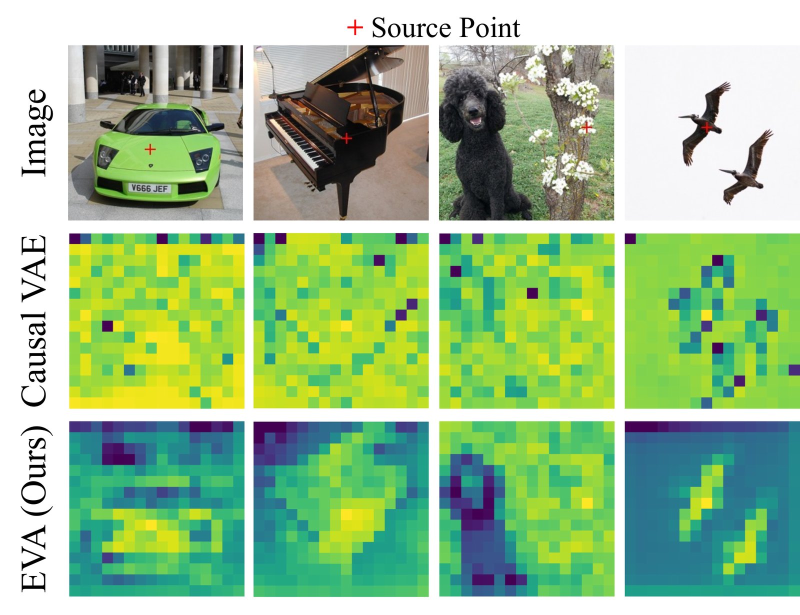
No loss here asks for semantics. EVA's posteriors still cluster by object, and I think the reason is the forecast: a latent that can be predicted from context is one where "more of the same thing" is a short step. The paper reads it the same way, as generation encouraging the model to learn semantics.

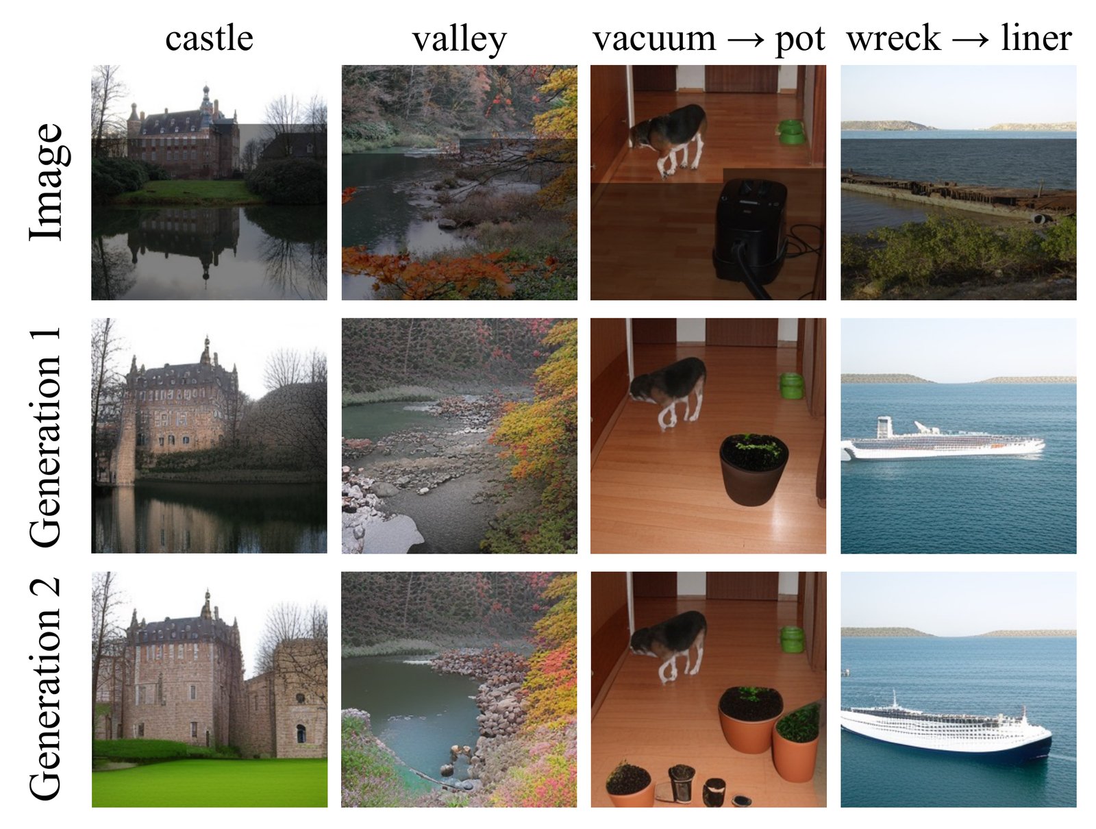
Prefix completion works for the same reason. Encode the first $t$ tokens of a real image, then sample the rest from the forecast chain. Changing the class label mid-image ("vacuum" to "pot", "wreck" to "liner") steers the completion.

expand

Where the paper and the release disagree

None of these changes the conclusion, but each will cost a reproducer an afternoon.

Start with the block counts. The paper describes EVA-S as "16 Transformer blocks each for encoder and decoder" at width 512, and EVA-L as 32 each at width 1024. The released weights say otherwise: I counted encoder_blocks.* and decoder_blocks.* indices in each safetensors header. EVA-S has 8 and 8, EVA-B 12 and 12, EVA-L 16 and 16. The repository's README table and its eva_small/eva_large factories agree with the weights. The paper's figures look like totals.

The audio latent is twice as wide as stated. The paper says VGGSound clips are "tokenized into 215 tokens with 32 channels". tasks/specs.py sets latent_shape=(64, 215), and the released VGGSound checkpoint's encoder_token_proj.weight is [768, 64]. The Stable Audio Open VAE's latent has 64 channels, so the code is the one to trust.

Then the configs. The EVA-L checkpoint on Hugging Face is eva-imagenet-large-64-ema, with latent size 64. That matches Figure 6b, and configs/imagenet/large_generate.yaml sets reparam_dim: 64. But configs/imagenet/large.yaml, the training config, sets 128. Running the training script as shipped does not produce the released model. The learning rate also differs from the paper's text. The paper says 1e-4. main_eva.py:80 multiplies that by the global batch over 256, MAR's convention, so on the paper's eight GPUs at 64 per GPU the actual rate is 2e-4. Finally, the README points at assets/vggsound_class_mapping.json, which is not in the repository. A class_mapping.json ships with the VGGSound checkpoint on Hugging Face instead.

Last, the objective is a weighted ELBO rather than the bound in Eq. 17. _kl_gaussian returns kl.mean() over all 128 latent dimensions, and the reconstruction is F.mse_loss averaged over 16 tokenizer channels. Relative to the summed bound in Eq. 17, the KL is weighted by 16/128, one eighth, against the squared error. And MSE is a Gaussian likelihood with a fixed variance anyway. In practice EVA is a $\beta$-weighted ELBO, which is how almost every working VAE is trained. The weight here comes from tensor shapes rather than a chosen hyperparameter. If you change reparam_dim, you also change the effective $\beta$. That could be part of why Figure 6a finds 128 better than 256.

What it doesn't do

The paper lists two limitations itself: latents are flattened into a 1D raster sequence, ignoring 2D structure, and the experiments stop at class-conditional ImageNet and VGGSound at moderate scale. I'd add three.

The first is that this is still a two-stage pipeline. EVA learns a VAE over the latents of another VAE: MAR's KL-16 tokenizer for images, Stable Audio Open's for audio. "No VQ-VAE or diffusion" is true; a VAE generating pixels it is not.

It is also strictly sequential, at 256 decoder steps per image, one token at a time. Each step is cheap, and the paper's timing compares it only with other one-token-per-step models. Masked and bidirectional generators emit many tokens per step, and the strongest of them are well ahead on FID. 7.68 for EVA-B and 6.04 for EVA-L are good for the parameter count and the speed, but they are mid-pack numbers, and to its credit the paper doesn't pretend otherwise.

And nobody has reproduced any of it yet. It is a single-author paper dated 5 October 2026, with weights published a day later. I did not run the code or the checkpoints either; everything here was read from the paper, the code and the safetensors headers.

Would I use it

As a generator for a product today, no. A diffusion or flow model on the same tokenizer is better, and the tooling around those is mature.

As an idea, yes, and I expect to see it again. Asking the encoder to make its latents predictable rather than merely compact is a small change with a large effect: 100.27 to 7.68 FID for 0.11% more parameters. It applies anywhere a VAE already sits under a causal model. Speech and audio codecs with an autoregressive generator on top are the obvious place, given that EVA already ties the diffusion heads on VGGSound at a fraction of the cost. The related bet runs through CSFM, which learns the source distribution of a flow instead of fixing it to Gaussian noise. It also connects to the latent-design arguments in GAE and Mage-Flow. The fixed $\mathcal N(0,1)$ keeps turning out to be a default nobody chose. And if you are thinking about where autoregression ends and diffusion begins, Set Diffusion maps that spectrum for discrete tokens, and the diffusion transformer page covers the backbone EVA's bidirectional competitors use.

How I checked

I read the paper's HTML version in full (v1, including Appendix B) and the project page. I read the Kaede Shiohara thread and replies through the fxtwitter mirror: the thread carries the paper and code links, and the replies add nothing beyond them. I shallow-cloned mapooon/EVA and read models/eva.py, engine_eva.py, main_eva.py, tasks/specs.py, the dataset loader and every config. Line numbers above are from that clone. I executed none of it.

For the weights, I read the safetensors headers of the five checkpoints under huggingface.co/mapooon with HTTP range requests. I summed tensor shapes for the parameter counts, counted block indices for the depths, and read each repository's metadata.json and config.yaml. The two widgets are my own constructions, labelled as such: a correlated-Gaussian toy for the prior gap, and hand-built predictors on the paper's toy spacing for the mode comparison. The numbers I quote from them come from running their arithmetic. MAR's comparison numbers are from its arXiv HTML, Tables 1 and 4. The repository's licence file is MIT. It is MAR's, still carrying MAR's copyright line, and the Hugging Face checkpoints declare no licence.