2026-10-06 · 20 min · explainer · training · pretraining · theory · backpropagation · optimization · transformers
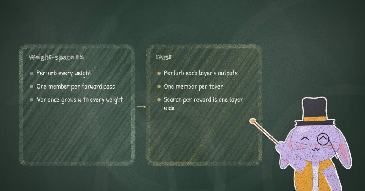
"Backprop has been the only credit assignment algorithm capable of training large neural nets." That is how Samip Dahal opens the thread announcing Dust, from Q Labs, written with Bishwas Mandal, Serdar Gülbahar and Akshay Vegesna. The claim that follows is that Dust is "the first zeroth-order method to pretrain transformers to approach and sometimes even exceed backprop with large amounts of computation", and that it is "on the order of 1,000 to 10,000x more compute efficient than EGGROLL".
Zeroth-order means the optimizer only ever sees loss values. That family has a well-earned reputation for collapsing in high dimensions, so this is worth taking apart.
I read the post, its appendix, and the released code (qlabs-eng/dust, MIT, commit 2fdb01b). I did not run it: the paper configuration wants eight GPUs per run. Numbers below are labelled reported (Q Labs' figure, not re-run), measured (I read or computed it from a file, the code, or the toy on this page), or reasoned (my arithmetic on the other two).
What a zeroth-order gradient is
Start with any loss over parameters. Nudge the parameters in a random direction by a small step . To first order,
One scalar, the loss change, tells you how much of the gradient lies along . Multiply it back onto and average over directions:
Because , the expectation of is the gradient. That is the evolution-strategies estimator of Salimans et al. (arXiv 1703.03864) and the random gradient-free method Nesterov and Spokoiny analysed. Evaluating as well and using the difference of the pair (antithetic sampling) cancels the even-order terms, so the curvature does not leak into the estimate.
The catch is variance. Each sample is the true gradient's component along one random direction plus everything else that direction carries. For an isotropic Gaussian, the error of has squared norm of roughly , so the cosine between estimate and truth is about
To get a cosine of one half you need evaluations. Dust's base model has 37.7M parameters (reported). Weight-space ES on it would need about 12.6M forward passes per update for a cosine of 0.5, and at 16,384 forward passes the cosine is about 0.02 (reasoned, from the formula above). That is the wall every weight-space method hits.
EGGROLL (arXiv 2511.16652) attacks the cost per member: it makes each perturbation a rank- matrix, so a whole population of perturbed models runs as one batched inference at up to 91% of plain inference throughput (reported, in its abstract). It does not change . Every member is still one sequence of the batch, and the population is still bounded by the forward passes you can afford.
Perturb the activations, not the weights
Dust moves the noise. Take one linear layer, , at token . Backprop's weight gradient for that layer is
The input is free: the forward pass already computed it. The only hard part is the output error , which backprop gets from the chain rule. Dust estimates it by jittering the layer's output instead: with , at every token, in one forward pass. The post writes the reward at token as the loss reduction there, plus the decayed reductions at later tokens that the jitter reaches through attention:
Here is the centred loss reduction at token , is the number of draws (one draw is one independent jitter of all tokens), and is a credit decay that is zero for everything except the attention internals. The last equation is the same outer product backprop forms. Only the source of the error differs. This is node perturbation, which Widrow and Lehr described in 1990 and Werfel, Xie and Seung analysed in 2003; the post cites both.
The textbook argument for node perturbation is dimension: a layer's output has numbers and its weights have . The post is candid that this argument, read naively, fails for a transformer. Noise on one sequence is a tensor, which has at least as many entries as the weight matrix once . If you reward that whole tensor with one scalar, you are back to searching a space as big as the weights.
What rescues it is the per-token reward. Each token's loss mostly reflects its own jitter, so each token's noise is scored by its own number. The search per reward is then -dimensional, and the tokens of a sequence are separate population members evaluated in the same pass. Q Labs calls that a virtual population. A sequence of 2,048 tokens is 2,048 members, where EGGROLL gets one.
Try it: three estimators, same forward passes
The widget below is a toy, not the paper's model. One linear layer, 32 tokens, a quadratic loss at each token. Three estimators get the same number of forward passes :
- weight-space ES, with antithetic pairs, so pairs, each scored by the summed loss;
- activation noise with one reward per pass: every token's output is jittered, and all of them are credited with the summed loss change;
- activation noise with one reward per token: Dust's direct draws with , each token's noise credited with its own loss change.
The two activation estimators rebuild the weight gradient exactly as Dust does, as . The curve is the cosine to the true gradient.
| estimator | searched per reward | cosine at K = 256 |
|---|---|---|
| weight-space ES (antithetic) | 256 (d × d weights) | 0.536 |
| activation noise, one reward per pass | 512 (T × d activations) | 0.511 |
| activation noise, one reward per token (Dust) | 16 (d per token) | 0.968 |
The toy reproduces the post's dimension argument (measured, one seeded run per width). At width 16, with 256 forward passes, weight ES reaches a cosine of 0.536 and the one-reward activation estimator 0.511, because the second searches 512 numbers per reward against the first's 256. They are equally hopeless. The per-token estimator is at 0.968 with the same passes. At width 64 the gap is wider: at 2,048 passes weight ES sits at 0.442, one reward per pass at 0.557, one reward per token at 0.984. The per-token curve barely moves as the width grows, because what it searches per reward is , not and not .
The toy is kind in two ways. Its token losses do not interact, so the per-token estimator suffers none of the cross-token interference attention creates in a real model; that interference is what most of Dust's engineering is for. And its loss is exactly quadratic, which flatters antithetic weight ES, since the pair difference is then exactly the directional derivative.
What the released code actually does
The repository is small: dust.py is 607 lines and model.py 201 (measured). The model is the modded-nanoGPT kind of decoder: eight pre-norm blocks of width 512, squared-ReLU MLP, rotary embeddings with normalised queries and keys, value embeddings on alternate blocks, a soft-capped untied head (reported in the appendix, and it matches model.py). It is the nanoGPT speedrun lineage. Nothing in dust.py calls backward(): the model is built with requires_grad_(False) and the update runs under torch.no_grad() (measured).
One update in DUST.step, as I read it:
- A clean forward caches every
LinearandEmbedding's input and output through forward hooks, plus the per-token losses. - Direct draws.
direct_errorssets a jittersigma * aon the chosen sites, reruns the forward, and computesreward = clean_loss - perturbed_lossper token. When several draws share one forward (the batch repeatednreptimes), the reward is centred across them; withnrep = 1it is not. The error estimate accumulates-reward * a / sigma. These rewards use the token's own loss only, so . The attention and MLP output projections (the "writers" into the residual stream) are jittered together in one stream, the MLP's first layer in another, all at . - Attention outputs, block by block, with in the first half and in the deeper half, because, in a code comment's words, "The deeper half moves the loss too little at 0.2 for a readable reward". These estimated errors become targets.
- Attention internals (queries, keys, values, the value-embedding gate and the value embeddings) never touch the loss.
local_errorsrecomputes only that block's attention from cached activations with a jitter and scores the change against the estimated attention-output error, the post's . Keys, values, gates and value embeddings sum the scores of later tokens decayed by ; queries keep their own token's score. - The head is jittered on the cached logits, one 256-column slab of the 4,096-token vocabulary at a time, recomputing only the cross-entropy from cached partial sums.
- The 2L residual-mix scalars are the only weights trained by weight-space ES, with two-sided pairs.
reassembleturns each error into a weight gradient withtorch.einsum('btd,bti->di', error, x), or a scatter-add for an embedding. Every estimate is divided by the token count, written into.grad, and SGD with momentum takes the step.
So the gradient with respect to the weights is not inferred from weight noise at all. It is the outer product backprop forms and the animation shows, with only the error vector coming from the population.
The population count is narrower than it sounds. In recipe(), at population 256 the writer and MLP-hidden streams each get 110 draws spread over the eight blocks (38, 32, 16, 10, 6, 4, 2 and 2, tilted toward the first blocks), the attention outputs 26 and the token embedding 10, which sums to 256 (measured). At 16,384 everything scales by 64: 7,040 + 7,040 + 1,664 + 640 = 16,384, matching the appendix's Table 3 (measured). The head's 65,536 slab draws and the attention-internal draws are on top of ; the post says they are a small share of an update's compute (reported).
One oddity: the token embedding trains at a learning rate of 1000 under SGD, for Dust and backprop alike (measured in make_optimizer, matching the appendix).
The results, checked against the tables
The setup (reported): FineWeb with a 4,096-token BPE tokenizer, batches of 8 sequences of 2,048 tokens, one epoch, SGD with momentum at a constant learning rate, three seeds per cell, every method tuned per token budget and population. In the released config, the 1M-token budget is 61 steps and the 10M budget 610 (measured).
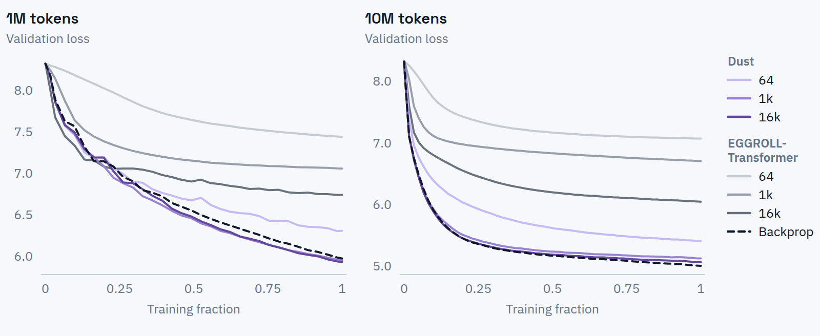
The headline ladder is Table 1 in the appendix. Test loss at the best-validation checkpoint (reported):
| Budget | Dust, 64 | Dust, 1k | Dust, 16k | Backprop | EGGROLL, 16k |
|---|---|---|---|---|---|
| 100k tokens | 7.240 | 7.151 | 7.170 | 7.216 | 7.263 |
| 1M tokens | 6.290 | 5.934 | 5.916 | 5.959 | 6.708 |
| 10M tokens | 5.397 | 5.111 | 5.049 | 4.989 | 6.033 |
| 20M tokens | 5.265 | 4.960 | 4.802 | 4.633 | 5.865 |
"Beats backprop at 100k and 1M tokens" holds in the table. The best Dust cell is 7.151 against 7.216 at 100k, and 5.911 (at 4k draws) against 5.959 at 1M, margins of 0.065 and 0.048 nats (reasoned). "Close at 10M and 20M" holds too, with gaps at 16k draws of 0.060 and 0.169 nats (reasoned). The 20M claim that the asymptote sits below backprop rests on a power-law fit through five cells that are still falling: limit 4.431, 95% interval 3.89 to 4.58, against backprop's 4.633 (reported). The post itself reads that as "evidence that the gap keeps closing with population rather than as a measured limit". So should you.
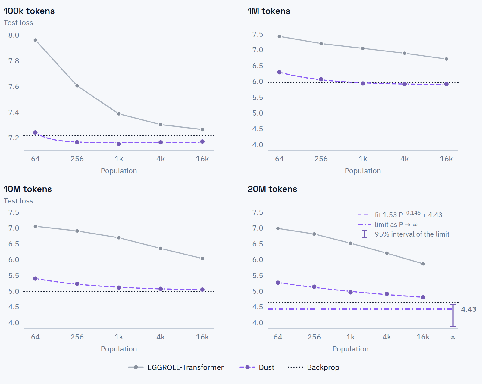
The EGGROLL comparison is two different claims. The measured one is in the table: EGGROLL at 16k forward passes never reaches Dust at 64 draws at any budget. At 100k tokens it is 7.263 against 7.240, 0.023 behind, which the post rounds to "within 0.02"; at 1M, 10M and 20M it is 0.4 to 0.6 nats behind (reported). The "1,000 to 10,000x" figure is not measured; the post says "based on our extrapolations". Appendix Table 2 extends EGGROLL's ladder by four kinds of fit to the population it would need to match Dust at 64 draws. The main fits put it between 3,100x and 23,000x that population. Refitting with one population left out widens the range to 54,000x at 10M, and one such refit at 1M never gets there at all (reported). Q Labs' own caveat is that, from 256 draws up, a Dust draw costs less than an EGGROLL forward pass, so the comparison is lenient to EGGROLL (reported).
Under Adam, at 1M tokens only, the shape repeats. Dust's power-law limit is 5.248 with an interval of 5.17 to 5.30, below backprop; EGGROLL's Adam ladder lands within 0.01 of its SGD ladder at every population (reported). That is one budget, and the Adam runs give the token embedding extra draws, about 1.4x the listed population in total.
Bigger models need fewer draws, up to a point
The claim I found most interesting is the one about size. The variance argument above says a bigger model needs a bigger population. Q Labs trained four sizes at a fixed 10M tokens: 2.0M, 7.3M, 38M and 243M parameters (2, 4, 8 and 16 blocks at widths 128 to 1024).
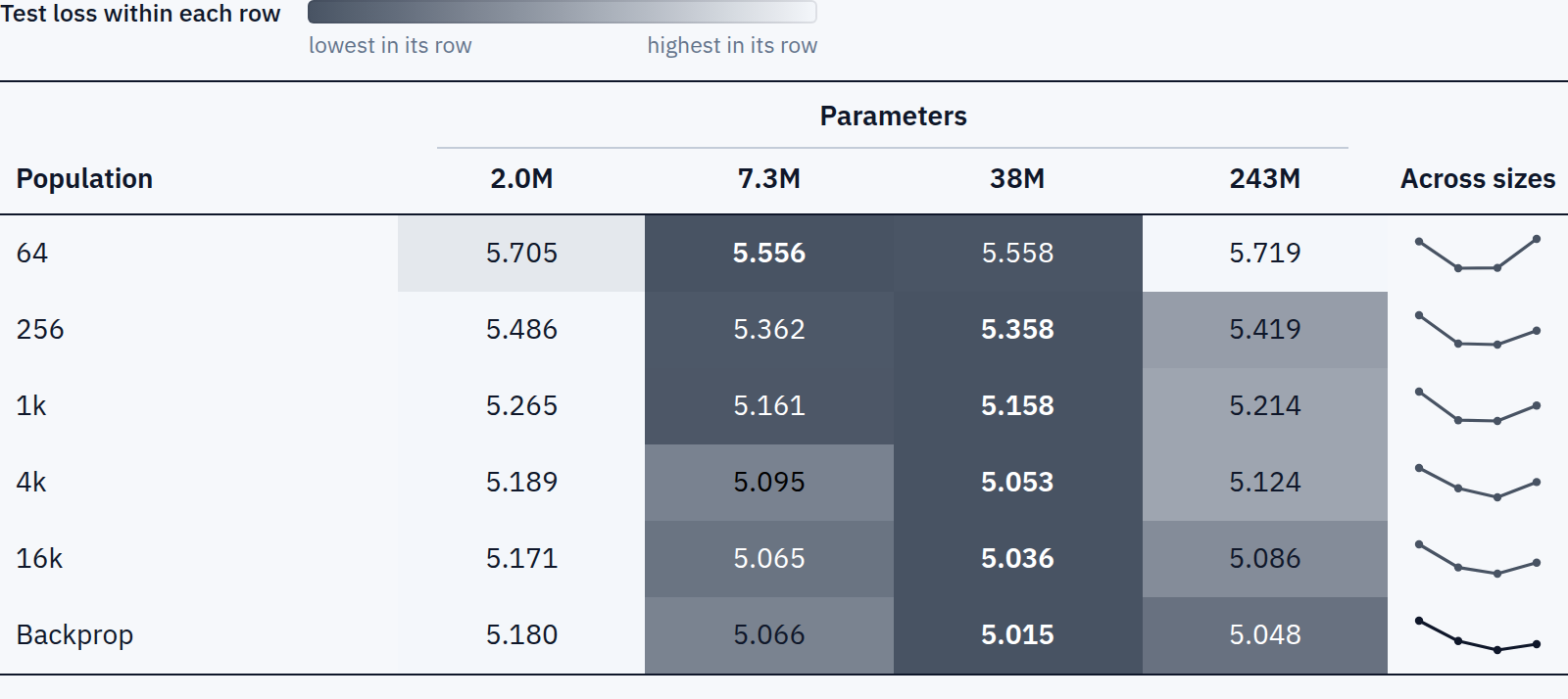
Read straight off the table (measured from the published cells):
- The 243M model beats the 2.0M model at four of five populations; at 64 draws it loses, 5.719 to 5.705. "Beats one 120x smaller at most population sizes" holds. The ratio is 121.5x (reasoned).
- The best size from 256 draws up is 38M, not 243M. The 243M model is worse than both 7.3M and 38M at every population. So loss falls with size "up to a point", as the post says, and the point is 38M at this budget.
- From 1k to 16k draws, the two larger models improve by 0.122 and 0.128 nats and the two smaller by 0.094 and 0.096, about 30% more (reasoned; the post says "about 30% more").
- The gap to backprop at 16k draws grows with size: Dust at 2.0M is 0.009 nats below backprop, at 7.3M 0.001 below, at 38M 0.021 above, at 243M 0.038 above (reasoned). The post calls this growth "barely noticeable".
Q Labs' reading is that overparameterization gives search "a bigger space with better geometry". My reading is narrower. Per-token rewards make the search dimension per reward the layer's output width, which for square layers grows roughly like rather than like , so the variance penalty for size is mild. A wider model is also a better model at a fixed token count, and that gain can outrun the penalty. One more caveat from the appendix: the size study predates the main protocol and uses the old token-embedding learning rate, chosen because at 1000 "backprop shows no clear separation between model sizes".
Backprop-like gradients, measured as a cosine
The last claim is that backprop-like gradients emerge from the population. Q Labs measured the cosine between Dust's estimate and the exact backprop gradient on the same batch, on backprop-trained checkpoints at 10M, 100M and 1B tokens, with populations from 64 to 128k.
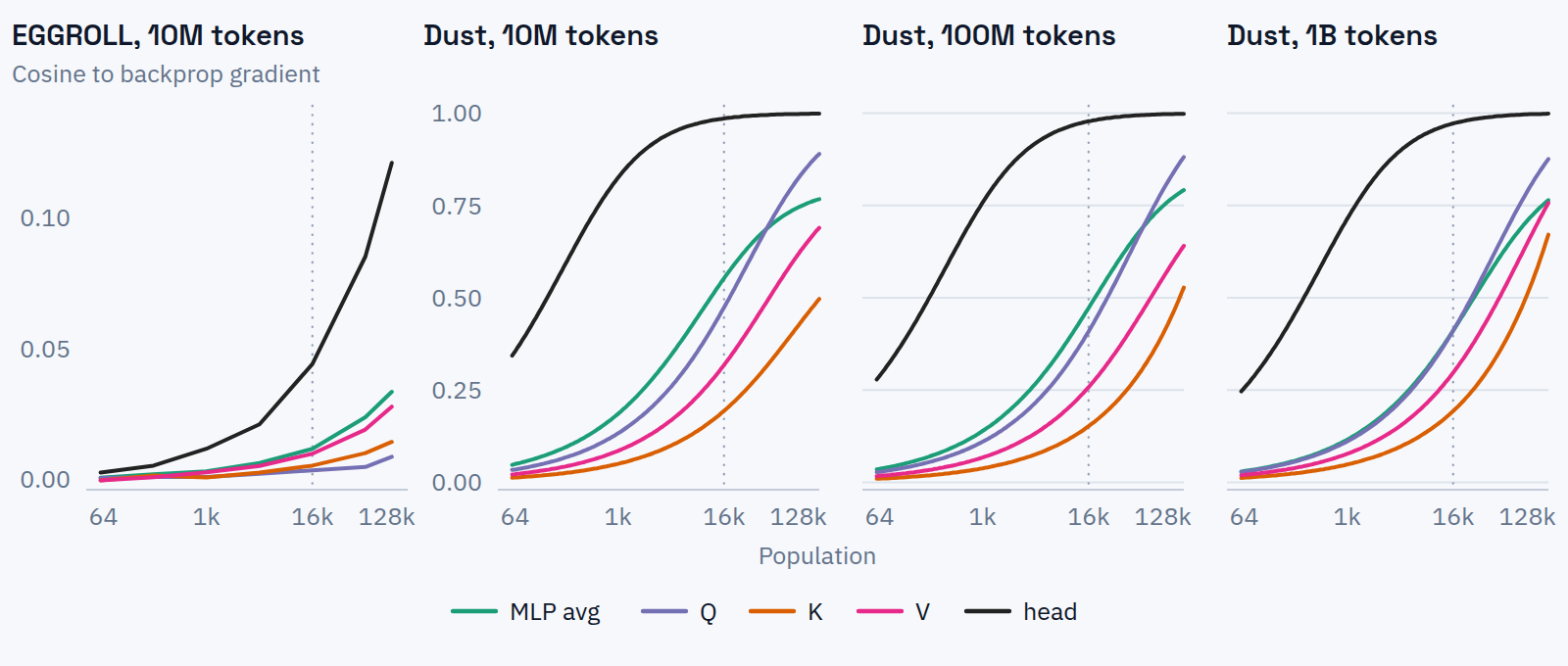
A two-parameter law, , fits each layer type with RMSE under 0.06 (reported). It is the same shape as the estimator variance above, with playing the effective dimension and a ceiling below one. Plugging the appendix's Table 8 fits for the 100M-token checkpoint into the law at the training population of 16,384 (reasoned): MLP output 0.51, attention output 0.57, token embedding 0.49, attention values 0.26, attention keys 0.16, and the head 0.98. The keys' fitted is 616,595, which is why their curve has barely left the floor at 16k. EGGROLL, measured the same way, stays below 0.05 at 128k for every layer type except the head (reported).
Two things to keep in mind. These are cosines on backprop's checkpoints, not along Dust's own trajectory. And a cosine of 0.5 is a modest alignment; SGD with momentum averages over steps, which is part of why it trains anyway. The post's further point, that Dust's gradients are "useful but different" and that the difference is sometimes better, is an observation from the ladders, not something the cosine study tests.
What it costs
This is where the result needs the most care. The post says it plainly: "We must have orders of magnitude more compute efficiency before Dust becomes a practical alternative to backprop at current levels of compute." Neither the post nor the code reports wall-clock time against backprop.
From the code I can estimate the forward work per update (reasoned). A draw at block reruns blocks through 8. With the 1M-token allocation at 16,384 draws, the writer and MLP-hidden streams, the attention outputs and the token embedding cost about 13,000 block-passes' worth, in units of one full eight-block forward. Backprop costs roughly three forwards' worth. That puts Dust at a few thousand times backprop's compute per update, before counting the head and attention-internal draws. At 256 draws the same arithmetic gives about 200 forward-equivalents, around 70x. The paper's eight-GPU runs split the draws across GPUs; they do not make them cheaper.
The regime is also early. The best losses here are 4.6 to 4.8 nats at 20M tokens, against a uniform-prediction loss of (reasoned). One reply to the thread made the point that at 5 nats most of the signal is still pushing unlikely tokens down, and that feature learning has barely started. The tuned grid matters too: backprop here is SGD with momentum at a constant rate, not a tuned Muon or AdamW schedule. The Adam ladder helps, but only at 1M tokens.
Where it sits
Dust is honest about its lineage. Node perturbation dates to Widrow and Lehr; GEMINI (Le Cun, Galland and Hinton, 1988) injected noise into hidden layers; Ren et al. scaled forward gradients with local losses; MeZO fine-tunes with forward passes alone; and Zoop used output perturbations for fine-tuning; a reply to the thread linking that paper said they tried "something very similar last year but only saw it working on finetuning". Another reply pointed to Nesterov's random gradient-free methods and to a functional version for infinite-dimensional spaces (arXiv 2512.20566), from one of the authors of the functional gradient descent paper covered here. That work is a related estimator, not a source for Dust.
What is new is the combination: per-token rewards as a population axis, separate passes per layer type to keep interference down, attention internals credited through an estimated local target, and a tuning loop that maximises cosine to backprop on one batch before any training. The post's motivation is not efficiency. It is that a search-based optimizer does not need differentiability, so it could train looped or program-in-the-loop models that backpropagation through time struggles with. None of that is tested here. On a smaller scale, the same trade, evaluations instead of gradients, shows up in Sakana's Fugu, where CMA-ES tunes a coordinator over ten thousand parameters.
What I want next: a budget where backprop gets below 4 nats, wall-clock next to backprop on the same GPUs, and a model only Dust can train. Until then, Dust is the best evidence I have seen that zeroth-order credit assignment can follow backprop through transformer pretraining, at a price that is still its main problem.