ZUNA 1.1: a channel-agnostic EEG foundation model

2026-07-17 · 10 min · eeg · foundation-model · diffusion · signal-processing · neuroscience · explainer

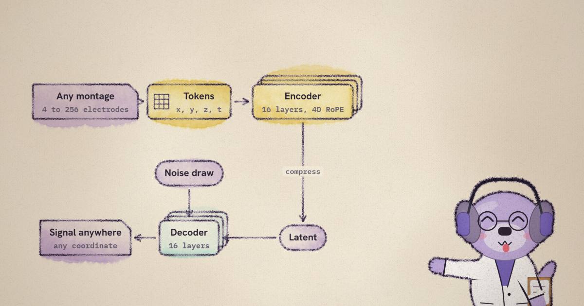
ZUNA 1.1, from Zyphra, is an EEG foundation model: a 380M-parameter transformer encoder–decoder diffusion autoencoder that reconstructs missing channels, denoises corrupted ones, and upsamples sparse montages to electrode positions that were never recorded. It is Apache-2.0, runs on a consumer GPU or a plain CPU, and — the part I find interesting — it is channel-agnostic: the same weights read a 4-electrode consumer headband or a 256-channel research cap, because it treats every electrode as a token at a physical coordinate, not a fixed slot in a montage.

There is no arXiv paper; this is a release across the Zyphra blog, the Hugging Face model card, and the GitHub repo (pip install zuna, plus a browser-based Cloud EEG Playground). It is a point release on ZUNA1 — same 380M parameters, a bigger and cleaner training corpus, and a handful of design changes that matter more than the version bump suggests.

The problem: no two EEG setups agree

EEG is a mess to model across datasets, and the mess is structural, not incidental. A clinical 10-20 montage has 19 electrodes; a sleep lab might run 6; a research cap runs 64, 128, or 256; a consumer headband runs 4. The electrodes sit at different scalp locations, sample at different rates, and are filtered differently. Worse, within a single recording, channels die, drift, or go noisy for part of a session and recover later. Most models paper over this by fixing a channel list and re-referencing every recording onto it — which throws away recordings that do not fit and cannot exploit the extra electrodes when they exist.

ZUNA's bet is to stop treating a recording as a fixed-width tensor and start treating it as a set of tokens, each tagged with where and when it was measured. Once the model keys on physical position instead of channel index, the montage stops mattering.

Channel-agnostic: an electrode is just a coordinate

The mechanism is a 4D rotary positional encoding. Each 0.125-second segment of one electrode becomes a token, and its position is the tuple $(x, y, z, t)$ : the electrode's 3D coordinate on the scalp plus a coarse time index. Attention applies rotary phases over all four axes, so "nearby" means nearby in space and time — the model learns that Cz and C3 covary because they are physically close, not because they happen to be channels 10 and 9 in some file.

That single choice is what buys channel-agnosticism. There is no learned per-channel embedding to run out of, so an arbitrary subset or superset of electrodes is just a different set of coordinates. Drop a region and the decoder fills those coordinates from the electrodes it still has; ask for coordinates that were never recorded and it predicts them the same way. Switch montages below and watch the same model span a headband and a dense cap:

channel-agnostic · one model, any montageillustrative

montage

stage

segment t (0.125s each)t=3

selected Cz · (x, y, z, t) = (0.00, 0.00, 1.00, 3)19 electrodes · 3 reconstructed

The same weights read every montage — a 4-electrode headband up to a 256-channel cap — because an electrode is just a token at position (x, y, z, t): its 3D scalp coordinate plus a coarse time index, fed to attention as a 4D rotary encoding. Nothing in the model is tied to a fixed channel list. Drop a region and the decoder fills those coordinates from the electrodes it still has; ask for coordinates that were never recorded and it upsamples to them the same way.

ZUNA 1.1 architecture: a 16-layer transformer encoder with RMS-norm blocks and 4D-RoPE self-attention feeds a latent into a 16-layer decoder whose self- and cross-attention blocks are conditioned by adaptive-RMS norm; the encoder takes clean and noisy EEG, the decoder emits the reconstructed signal. — The encoder–decoder. A 16-layer encoder maps clean context to a latent; a 16-layer decoder cross-attends to it and denoises, with 4D-RoPE over (x, y, z, t) on every attention block and adaptive-RMS norm carrying the latent into the decoder (Zyphra, ZUNA 1.1, 2026).

Inside the model: a diffusion autoencoder

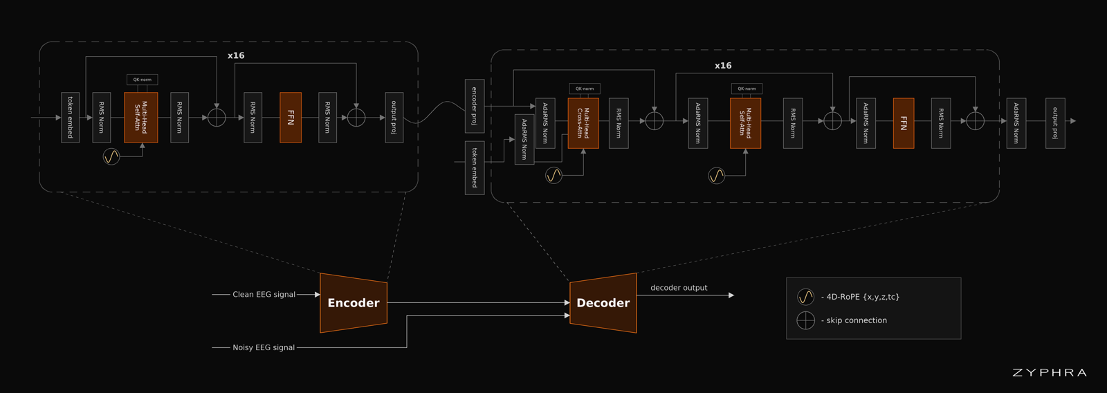
The architecture is two transformer stacks. The encoder reads the clean context and compresses it to a latent. The decoder cross-attends to that latent and produces the signal at the requested coordinates. The latent is injected into every decoder layer through adaptive-RMS norm — the latent sets the per-layer scale of the normalization, which is a cheap, stable way to condition a deep stack on a global summary (the same conditioning trick diffusion image models use for the timestep).

The decoder is trained with a rectified-flow objective rather than a plain regression loss, and this is the right call for reconstruction. Filling a missing channel is genuinely uncertain — many signals are consistent with the surrounding scalp — so a model trained to minimize mean-squared error returns the blurred average of all of them. A generative decoder instead returns a sample from the plausible set. Rectified flow makes that sampling cheap: it learns a straight-line transport from a noise draw to the data. With noise $x_0$ and target signal $x_1$ , the interpolant and its velocity are

x_\tau = (1-\tau)\,x_0 + \tau\,x_1, \qquad \frac{dx_\tau}{d\tau} = x_1 - x_0,

and the decoder regresses a velocity field $v_\theta(x_\tau, \tau)$ onto that constant velocity $x_1 - x_0$ . At inference you draw $x_0$ and integrate the field from $\tau=0$ to $\tau=1$ . Because the target path is a straight line, few integration steps get you most of the way — which is why this runs on a CPU. Drag the scrubber:

diffusion autoencoder · encode → latent → rectified-flow decodeillustrative

task

jump

pipeline (drag) · rectified-flow decoderesidual (illustrative) 0.00

Each 0.125-second segment (32 samples at 256 Hz) becomes one continuous-valued token. The encoder compresses the clean context into a latent, which conditions every decoder layer through adaptive-RMS norm. The decoder is trained with a rectified-flow objective: it learns a straight-line transport from a noise sample to the true signal at the requested coordinate. Drag τ from 0 to 1 and the reconstruction (solid) walks off the noise field and onto the clean target (dashed). The same decoder fills a missing channel, cleans a noisy one, or predicts a position that was never recorded — only the conditioning changes.

The same decoder does all three jobs — reconstruct a missing channel, denoise a noisy one, upsample to a new position — and only the conditioning changes. That is the payoff of framing everything as "predict the signal at these coordinates given those."

Training: corruption on purpose

The corpus roughly doubled over ZUNA1, from about 2M to 3.5M channel-hours of public EEG. Two things about how it was prepared are worth noting. First, quality is scored per channel, per second, so a channel that is clean for most of a session and noisy for a stretch is used where it is good instead of being dropped whole. Second, each recording is kept in two filter variants — a bandpass at 0.1–45 Hz and a minimally processed version (0.01 Hz high-pass plus a notch for line noise) — so the model sees both heavily and lightly filtered signal. Inputs are variable length, 0.5 to 30 seconds, bucketed into four bins so short clips are not wasted padding a long window.

The interesting part is that the model is trained to reconstruct under four distinct corruption patterns, not one. This is the whole reason it generalizes to messy real-world recordings:

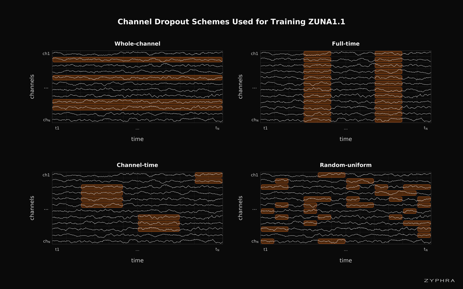
Four EEG channel-dropout schemes shown as multi-channel traces with masked regions highlighted: whole-channel (entire rows removed), full-time (vertical time slices across all channels), channel-time (rectangular space-time blocks in some channels), and random-uniform (scattered short segments). — The four dropout schemes the decoder is trained to invert — whole-channel (dead electrodes), full-time (dropouts across all channels), channel-time (localized space-time gaps), and random-uniform (scattered artifacts) (Zyphra, ZUNA 1.1, 2026).

Whole-channel dropout teaches it to rebuild a dead electrode from its neighbors. Full-time dropout — a gap across every channel at once — teaches temporal inpainting. Channel-time dropout is the realistic case: a cluster of electrodes goes bad for a window. Random-uniform scatter mimics muscle artifacts and momentary failures. Because training mixes all four, the model handles almost arbitrary space-time masks at inference, which is exactly what reconstruct_fif() exposes — it auto-detects MNE bad channels and BAD_ annotations and repairs them.

Results: reconstruction as channels drop

The metric is normalized mean-squared error between the held-out true signal and the reconstruction,

\mathrm{NMSE} = \frac{\lVert \hat{x} - x \rVert_2^2}{\lVert x \rVert_2^2},

where 1.0 is the trivial "predict zero" baseline and lower is better. The baseline to beat is MNE's spherical-spline interpolation, the classical way to rebuild a missing electrode from a smooth fit over the others. Zyphra publishes the comparison as figures, not tables, so the numbers below are read off the plots and are approximate.

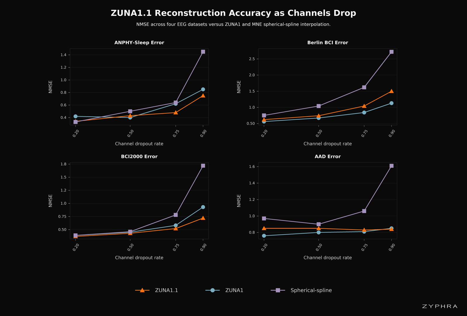
Four line plots (ANPHY-Sleep, Berlin BCI, BCI2000, AAD) of reconstruction NMSE versus channel dropout rate from 0.2 to 0.9. ZUNA1.1 and ZUNA1 curves stay low and close together while the spherical-spline curve rises sharply at high dropout, exceeding 2.5 NMSE on Berlin BCI. — Reconstruction NMSE as the fraction of dropped channels grows, across four datasets. Both learned models stay flat; classical spline interpolation blows up once most channels are missing (Zyphra, ZUNA 1.1, 2026).

At 20% channel dropout everything is close — NMSE around 0.4 to 0.6 across the four datasets, because with most electrodes present even a spline does fine. Push to 90% dropout and the spline blows up (Berlin BCI reaches roughly 2.7, i.e. worse than predicting silence) while ZUNA1.1 and ZUNA1 hold near 1.0 to 1.5. That widening gap is the headline: the learned prior degrades gracefully as information disappears; the classical interpolant does not.

ZUNA1.1 versus ZUNA1 is, honestly, a wash — ZUNA1.1 is a touch better on ANPHY-Sleep and BCI2000 and marginally behind on Berlin BCI and AAD. That matches Zyphra's own claim: better or essentially equal NMSE at the same 380M parameters, with the real gains going to stability and the broader input regime rather than raw accuracy.

The more realistic test deletes a whole brain region and rebuilds it from the other seven:

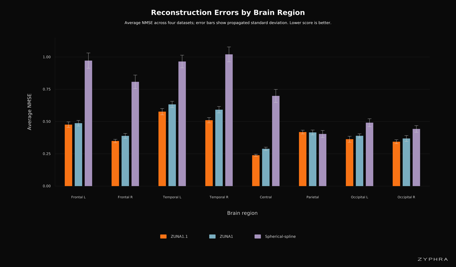
Grouped bar chart of average reconstruction NMSE by brain region (frontal, temporal, central, parietal, occipital, left and right) with error bars, comparing ZUNA1.1, ZUNA1, and spherical-spline. ZUNA1.1 and ZUNA1 bars are similar and low; spherical-spline is much higher for frontal and temporal regions. — Region-occlusion reconstruction: delete an entire region, rebuild it from the rest. The two learned models are close and both far below spline in frontal and temporal cortex; the gap narrows over parietal, where a smooth interpolant is already a decent model (Zyphra, ZUNA 1.1, 2026).

Here the two learned models track each other closely and both crush the spline in frontal and temporal regions (spline around 0.8 to 1.0 NMSE, ZUNA around 0.35 to 0.6). The three converge only over parietal cortex, where the field is smooth enough that a spline is already a reasonable prior. Central electrodes are the easiest — every model does well — because they are surrounded by neighbors on all sides.

Where it breaks

Two more honest limits. The evaluation is four datasets and F32 weights; generalization past those recording conditions is asserted, not shown. And rectified-flow decoding is iterative — CPU inference works, and it is cheap because the transport path is straight, but latency still scales with how many sampling steps you take, so "runs on a CPU" and "real-time" are not the same claim.

The take

The reframing that pays off is spatial. Making position, not channel index, the thing the model keys on is the whole idea, and 4D RoPE over $(x, y, z, t)$ is a clean way to do it. It is the same move that made vision transformers resolution-flexible, applied to the scalp — and it is what lets one set of weights span a headband and a 256-channel cap and interpolate to electrodes it never saw.
The diffusion-autoencoder choice fits the problem. Reconstruction is genuinely uncertain, so a generative decoder that samples a plausible signal is more honest than a regressor that returns the blurred mean. Rectified flow keeps that sampling cheap enough to run without a GPU.
It is built to be used, not admired — Apache-2.0, pip install zuna, a browser playground, and an MNE-friendly reconstruct_fif() entry point. The win over classical interpolation is decisive; the win over ZUNA1 is a tie, and Zyphra says so. Both are worth saying out loud.

Sources: the ZUNA 1.1 release, the Hugging Face model card, and the GitHub repo. Figures are from Zyphra's release; NMSE values are read off the published plots and are approximate, since exact tables were not released. Released 2026-07-16 under Apache-2.0.