2026-10-17 · 18 min · time-series · benchmarks · calibration · transformers · synthetic-data · small-models · licensing
A 1:46 narrated explainer, drawn in code. Every number and picture in it is this article's own; the sources are below.
› transcript
Hi, I'm Galloon! Timestral reads a stream of numbers and answers with a spread of possible futures. Here is how. Cut the history into patches, read them causally, and let separate forecast tokens ask for the future. First, the series becomes tokens. Cut it into patches of thirty-two steps. Each patch is a token. Scale each patch by what came before it, never after. Squash it, so a huge spike arrives small. And flag every missing value, so a gap stays a gap. The patches enter a twenty-four layer trunk. Each one reads only itself and earlier patches. Then come forecast tokens, copies of one learned vector. They read the whole context. The context never reads them. A head turns each forecast token into twenty-one quantiles per step, built so they cannot cross. Every fourth layer also looks across the series' other variables. Each quantile is trained with the pinball loss. Truth above the forecast costs tau per unit missed. Truth below costs one minus tau. So the forecast settles where a fraction tau falls under it. On two shared CPU threads, even the full context took six and a half seconds. It is only about a thousand tokens. The benchmark score, rebuilt from the leaderboard's own files, matches the card exactly. So remember: thirty-two thousand steps is only about a thousand tokens. That is why it runs on a CPU. Patches scaled by the past, forecast tokens that ask for the future, and quantiles that cannot cross. Every source is in the full article. I'm Galloon. Bye!
Why read this
Essentialtop 10%Timestral's patching, masks and quantile head from the code, a CPU run with timings and errors, and two leaderboards recomputed from raw files.
- Checked against the source
- Runs on a laptop CPU
- Interactive explanations
LLM architectureCustom licencePractitioner model
How this was scored
- Is it new?
- 2 of 3: A real new idea, method or capability
- Can I trust it?
- 3 of 3: Reproduces the headline result, or shows from primary files it is wrong
- Can I run it?
- 3 of 3: Open, permissive, runs on reader hardware with instructions
- Will I understand it?
- 3 of 3: Mechanism carried by interactives built from real code or data
- Can I act on it?
- 2 of 3: A concrete recipe, numbers or comparison
- Will it last?
- 2 of 3: A reference for a year or more
- Does it affect many?
- 2 of 3: A widely used model, tool or lab release
- Only here?
- 2 of 3: A teardown or measurement few others did
Score 84 of 100, ranked 8 of 577 rated articles. Each question is answered 0–3 by hand, and a 3 is rare. How articles are scored
On 15 October Mistral put a time-series model on Hugging Face. The announcement that reached me, via HuggingPapers on X, was one line: "State-of-the-art zero-shot forecasting across 3 major benchmarks, with 21 quantiles and up to 32k context."
Every part of that sentence hides a question. What is a token when the input is a stream of floats? 32k of what? What are 21 quantiles for, and how do you score them? Which three benchmarks, against whom?
There is no paper yet ("Tech report: coming soon!", says the card). There is something better for my purposes: a standalone inference package of about 1,700 lines of Python, Apache-2.0, that needs only PyTorch, NumPy, safetensors and huggingface_hub. So I read it, downloaded the weights, and ran it.
- task
- time-series-forecasting
- library
- timestral
- license
- other
- safetensors
- 1 shard
- largest file
- 837.3 MB
- files
- 6
- downloads
- 1.5K
- likes
- 78
repo last modified 2026-10-15
- license
- Apache-2.0
- branch
- main
- tests
- 1 file
- source
- 83.3 kB
- commit date
- 2026-10-15
by size of tracked source at this commit, file counts in brackets; docs, data and vendored trees excluded
local clone, 2026-10-17 at a534bdb — branch, commit, commitDate, fileCount, hasTests, languages, license, licenseFile, shallow, testFileCount
shallow clone: counts describe the pinned tree, not the history
Labels, as usual: measured means I computed it from a file or a run; reported is Mistral's or a leaderboard's figure that I did not reproduce; reasoned is my arithmetic on the other two.
A series is not a sentence
A language model's input is already discrete. A time series is not, and it has a worse problem: scale. The same model has to read a CPU-utilisation trace between 0 and 1, airline passengers in the hundreds, and an electricity meter in the millions. And unlike a document, one series can drift by an order of magnitude over its own history.
Earlier models answered this in different ways. Chronos quantises scaled values into a vocabulary of bins and trains a language model on the bin ids. Kronos does the same for candlesticks with a learned binary code. Timestral does not discretise at all. It follows the PatchTST and TimesFM line: cut the series into fixed-length patches, normalise each patch, and project its raw numbers into a vector with a small MLP. A patch is a token.
The details are in src/timestral/model.py and scaler.py, and three of them matter.
Patches are 32 steps (measured, config.json: "patch_size": 32). A context that is not a multiple of 32 is left-padded with zeros that are marked missing.
Normalisation is causal, per patch. Each patch is shifted and scaled by the mean and standard deviation of every observed value from the start of the series up to the end of that patch, computed as a running Welford sum in float64. A patch never sees statistics from its own future. The scaled values then pass through asinh, which is linear near zero and logarithmic in the tails, so a spike ten standard deviations out arrives as about 3 rather than 10:
# scaler.py: apply_affine_asinh_masked
scaled = (data - loc) / scale
scaled = scaled.masked_fill(~observation_mask, 0.0)
scaled = torch.where(observation_mask, scaled.asinh(), scaled)
Missingness is an input channel. The patch embedding sees 64 numbers per patch: the 32 scaled values and 32 flags saying which of them were missing (measured: patch_proj.hidden_layer.weight is [3072, 64]). A NaN in your data becomes a zero with a raised flag, not a guess.
That last point is how the card's two numbers relate. "Up to 32,768 historical time steps" is 1,024 patches, so the transformer never sees a sequence longer than 1,024 context tokens plus at most 32 forecast tokens (reasoned, from context_length: 32768, patch_size: 32 and block_size: 32). A 32k-step context sounds like a long-context model. In tokens it is a short one. That is also why it runs on a CPU, as we will see.
Where the 209M parameters live
The card says 24 layers and width 768. The safetensors header says more. I read it with two HTTP range requests, without downloading the 837 MB file: 203 tensors, all float32, 209,312,256 parameters (measured).
| Component | Parameters | Share |
|---|---|---|
| 24 SwiGLU MLPs (768 → 2 × 2,048 → 768) | 113,246,208 | 54.1% |
| 24 time-attention sublayers | 70,778,880 | 33.8% |
| 6 variate-attention sublayers | 17,694,720 | 8.5% |
| Quantile head (768 → 3,072 → 672) | 4,939,776 | 2.4% |
| Patch embedding (64 → 3,072 → 768) | 2,609,664 | 1.2% |
| RMSNorm scales and the forecast-query vector | 43,008 | 0.0% |
All measured from the header; shares are reasoned. Each attention sublayer is 2,949,120 parameters, five 768 × 768 matrices: the fused Q, K and V, the output projection, and a sigmoid gate that multiplies the attention output before the projection (time_attn_gate: "sdpa_sigmoid"). There are no biases anywhere in the trunk.
The two kinds of attention are the interesting part. config.json has a block_schedule of 24 entries: three "time" layers then one "time_variate", repeated six times (measured). A time layer attends along the patches of one series, with rotary position embeddings on half of each 64-dimensional head (rope_partial_factor: 0.5; see the RoPE explainer for what the rotation does). A time_variate layer does that and then a second attention across the variates of the same series at the same patch, with no position encoding, because variates have no order. That is how a pump's temperature can inform its pressure forecast: six times in the stack, every row of a series looks sideways at the others.
Covariates ride the same mechanism. Each row gets a role: target, past-only covariate, or known-future covariate. The masks in masks.py let covariate rows pass information to targets but never read them, and only known-future covariates are visible over the horizon. A holiday calendar can inform the forecast without the target leaking into anything.
Forecast tokens, not masked patches
How do you get a forecast out of a causal encoder? The common answer, which Mistral's blog attributes to Toto 2.0 and TimesFM-3, is to append masked patches and train the model to fill them in. Mistral's objection (reported, from the blog post) is that the values being forecast then look exactly like missing values, and are lost as context for later forecasts.
Their alternative is called Decoupled Horizon Forecasting. In code it is short. The sequence is [Enc ; Dec]: the context patches, followed by h copies of one learned vector, representation.forecast_query, 768 numbers (measured). The copies differ only by their rotary position. Each one is a question: "what are the 32 values at this offset?" The time-attention mask is what makes it work:
- context patches read themselves and earlier context patches (causal);
- the context never reads a forecast token;
- each forecast token reads every valid context patch, and the forecast tokens before it.
The widget below draws that mask from the same rules as build_forecast_time_mask. Rows are queries, columns are keys. Slide the padding to see left-padded patches drop out as keys. The lower half does the real-size arithmetic: how many tokens your history becomes, and how many decode blocks a horizon needs.
Since the history stays in the sequence untouched, every observed value in training is both a target for some forecast token and context for later ones. That is the claimed advantage: training horizons and missing-data augmentation can be tuned separately. I cannot check the training claim without the report. The inference side matches the description.
A horizon longer than 32 patches (1,024 steps) is decoded block by block. After each block, the median forecast is appended to the context as if it were observed, and the next block runs (measured, _block_ar_decode). There is no KV cache in this package: each block reruns the whole sequence.
One more subtlety. Forecasts come out in the normalised frame of the last context patch. But in training, horizon patch j was normalised with statistics that include the true values of patches before it. At inference those values do not exist, so advancing_block_frames substitutes the block's own predicted medians, re-deriving a running mean and scale patch by patch, and re-denormalises each horizon patch in that "advancing" frame. It is the kind of train-inference mismatch fix that only shows up in code.
21 quantiles, and why they cannot cross
The head maps each forecast token to 672 numbers (measured: head.projection.output_layer.weight is [672, 3072]), which is 32 steps × 21 quantile levels: 0.01, 0.05, then every 0.05 up to 0.95, and 0.99.
Predicting 21 numbers independently invites a classic bug: the 0.6 quantile comes out below the 0.55, and your 80% interval has negative width. monotone_quantiles rules it out by construction. The median output is free. Every other level is the median plus or minus a cumulative sum of non-negative increments, each 3.0 × Δp × softplus(raw), where Δp is the probability gap to the next level inward (measured; quantile_width_factor: 3.0 in the config). Softplus is never negative, so the quantiles are sorted before they leave the network.
The training loss is reported, not visible in an inference package: "a pinball loss over 21 quantiles, a discrete approximation of CRPS" (blog). For a quantile level , true value and prediction , the pinball loss is
It charges per unit when the truth lands above the prediction and when it lands below. Minimising it over many samples pushes to the point where a fraction of outcomes fall below: the -quantile. The continuous ranked probability score is , so averaging over a grid of levels approximates it. That is exactly what the leaderboards report as CRPS or WQL, divided by the sum of the absolute targets to make it scale-free.
At inference the forecaster adds two tricks of its own, both on by default (measured, forecaster.py). Symmetric averaging forecasts the series and its negation, reflects the second forecast back (-Q(1 - p)), and averages the two. It doubles the compute. Non-negative clipping clamps the forecast at 0 when the whole context is non-negative.
Running it on two CPU threads
The repository's own test suite builds random tiny models; nothing in it needs the weights. So I installed the package from the clone into a Python 3.12 venv with CPU-only PyTorch 2.14.1, downloaded the 209M checkpoint (799 MB on disk) and ran it on a shared cloud VM: an Intel Xeon at 2.1 GHz, torch.set_num_threads(2), nice -n 19, other jobs running. Treat the timings as an upper bound.
Latency against context length
A 96-step forecast from the end of ETTh1's oil-temperature column (or, past its 17,420 rows, a seeded random walk), minimum of five runs after a warm-up (measured):
| Context (steps) | Patches | One pass | With symmetric averaging |
|---|---|---|---|
| 128 | 4 | 0.117 s | 0.260 s |
| 512 | 16 | 0.144 s | 0.296 s |
| 2,048 | 64 | 0.267 s | 0.527 s |
| 8,192 | 256 | 0.756 s | 1.517 s |
| 16,384 | 512 | 1.453 s | 3.155 s |
| 32,768 | 1,024 | 3.108 s | 6.483 s |
With the defaults, a forecast from 8,192 steps took 1.517 s and one from the full 32,768 steps took 6.483 s. Symmetric averaging costs almost exactly 2x, as the code says it should. Cost grows close to linearly with context: doubling from 16,384 to 32,768 steps takes 2.1x (reasoned). At 1,024 tokens, attention's quadratic term is still small next to the MLPs, which hold 54% of the weights. A 32k-step context is cheap because it is a 1k-token context.
Mistral reports 140 ms for "one day ahead from three weeks of 15-minute history", 2,016 steps of context and 96 of horizon, on "a standard server CPU with 8 threads". My closest row is 0.527 s with the default symmetric averaging on 2 threads. Four times the threads would land near their figure if scaling were linear, which I did not test (reasoned).
Peak resident memory was 1,837 to 1,846 MB in every run, whatever the context (measured, ru_maxrss in a fresh process per run). The context barely registers; the weights dominate. Python and PyTorch take about 230 MB before loading, and the load itself adds about twice the 799 MB checkpoint, because load_model builds a randomly initialised model and then copies a second, loaded state dict into it (reasoned, from loading.py).
Error against seasonal naive
I held out the end of three classic public series and forecast it with the full history as context. The baseline is seasonal naive: repeat the last season. MASE divides the mean absolute error of the median by the in-sample seasonal-naive error over the training part; WQL is the CRPS-style score above over the levels 0.1 to 0.9, which is what GIFT-Eval uses (both measured, my scoring code).
| Series | Context | Horizon | MASE, Timestral | MASE, naive | WQL, Timestral | WQL, naive | 80% band covers |
|---|---|---|---|---|---|---|---|
| ETTh1 oil temperature (hourly) | 17,324 | 96 | 0.258 | 1.347 | 0.0687 | 0.3349 | 96 of 96 |
| ETTh1 high useful load (hourly) | 17,324 | 96 | 0.952 | 1.680 | 0.2273 | 0.5054 | 73 of 96 |
| Melbourne daily minimum temperature | 3,590 | 60 | 0.620 | 0.928 | 0.1179 | 0.2137 | 50 of 60 |
| Airline passengers (monthly) | 120 | 24 | 1.193 | 2.494 | 0.0544 | 0.1575 | 13 of 24 |
On every series the model beats the baseline by a wide margin: WQL is between a fifth and just over half of seasonal naive's. More context helps on the long hourly series. Cutting ETTh1's oil-temperature context to the last 512 steps moves MASE from 0.258 to 0.321 and WQL from 0.0687 to 0.0801; 8,192 steps gives 0.267 and 0.0698 (measured). On the temperature series, 512 steps instead of 3,590 moves MASE from 0.620 to 0.711.
Symmetric averaging is not free accuracy, either. Turning it off on the long ETTh1 run moved MASE from 0.258 to 0.276 but WQL from 0.0687 to 0.0670, slightly better. On airline passengers it helped both: MASE 1.419 and WQL 0.0666 without it (measured). One window each, so this is texture, not a finding.
The calibration column is the honest one. The 80% band should contain about 80% of the outcomes. On oil temperature it contained all 96, and the 50% band held 86 of 96: the bands are too wide. On airline passengers it held 13 of 24 and the 50% band 2 of 24: the 1960 traffic ran above the median for most of the year, and the band was too narrow to catch it. Too wide on one series, too narrow on another, with one window each, is what single-window calibration looks like. It is a reason to backtest on your own data, not a verdict.
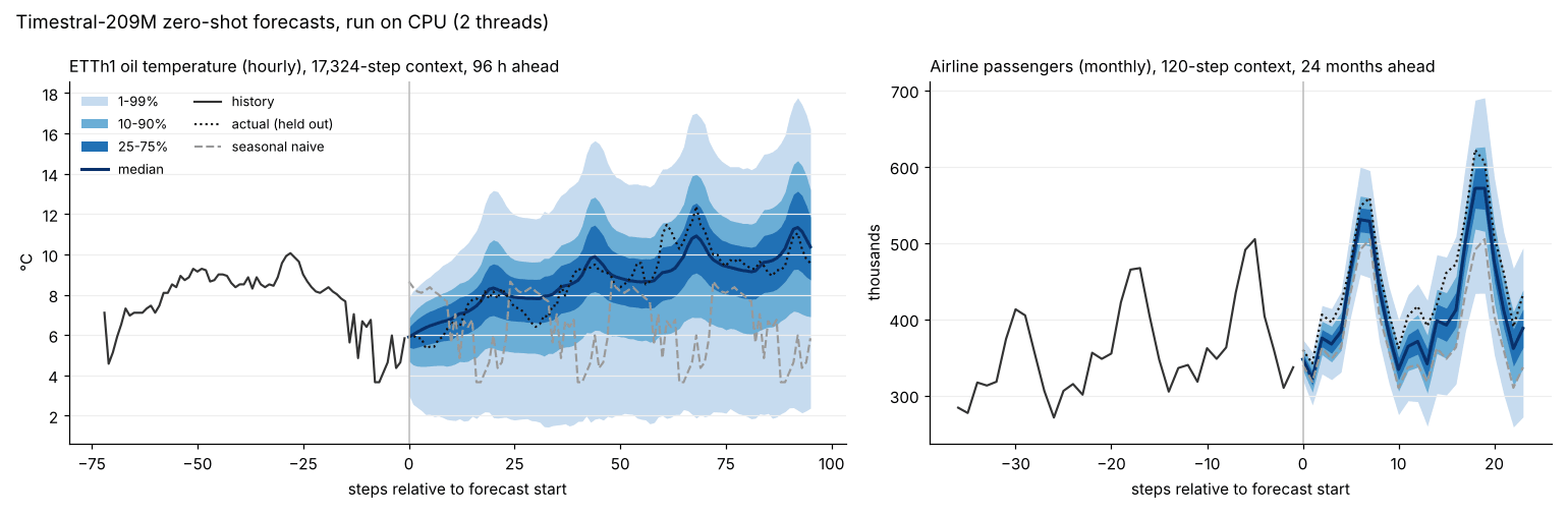
The widget holds the raw output of those two runs: all 21 quantiles at every step. Pick which bands to draw, slide along the horizon, and choose a quantile level to see its pinball loss against the naive forecast's, and how many actuals fell below it.
A few things worth trying in it. On oil temperature at = 0.9, the mean pinball loss over the 96 hours is 0.231 °C against naive's 2.301 (measured). On airline passengers at = 0.1 the two are nearly tied, 7.091 against 7.125 thousand passengers, while at = 0.5 the model is twice as good, 17.049 against 35.625. At = 0.1 a forecast below the truth pays only 0.1 per unit of miss. Naive repeats 1959, which was lower than 1960, so it sits below the truth almost everywhere and pays very little; a low quantile has almost no room to beat it.
A caveat that applies to every number in this section: ETTh1, the airline series and the Melbourne temperatures are among the most-copied datasets in forecasting. Mistral says pre-training was "purely synthetic" and post-training used "a mix of real and synthetic data", without listing the real data. I cannot rule out that some of these series were in it.
The three benchmarks, rechecked
The three benchmarks are GIFT-Eval (97 dataset configurations), fev-bench (100 tasks) and TIME (98 tasks), per the repository's README (reported). All three score probabilistic and point forecasts as above, divide each task's score by seasonal naive's, and aggregate with a geometric mean, so 0.446 on GIFT-Eval's CRPS means the forecasts are, in geometric mean, about 55% better than repeating the last season (reasoned). fev-bench reports the same thing as a skill score, 100 × (1 − geometric mean).
Two of the three publish their raw per-task results, so I recomputed them rather than trusting the table.
GIFT-Eval. The leaderboard Space stores one all_results.csv per submission. I downloaded all of them and rebuilt the overall scores. Timestral-209M's 0.658 MASE and 0.446 CRPS come out exactly, over all 97 configurations (measured). Of the 151 submissions with every configuration, 75 are marked zero-shot or pretrained with no test-data leakage; on CRPS, Timestral-209M is first among them, with Timestral-123M second at 0.448 and t0-gamma third at 0.452 (measured). It also has the best average per-configuration rank on both MASE and CRPS among those 75.
It is not first on every number. Morpheus-2.0, submitted by JP Morgan Chase as a pretrained model the same day, has a lower geometric-mean MASE: 0.646 against 0.658, with a worse CRPS of 0.455 (measured). Its entry has no model link, no code link, and says replication code is not available, which is presumably why Mistral's charts compare against "public models". Mistral's blog counts 83 comparable entries; my count of 75 excludes partial submissions and a few whose result folders I could not fetch. Across all 151, eleven entries have a lower MASE than Timestral-209M: Morpheus-2.0 and ten agentic systems, led by EXAONE-Forecast-Agent at 0.610 MASE and 0.419 CRPS (measured). Those are pipelines, often wrapping several foundation models; a single checkpoint is a different product.
fev-bench. The results live in the autogluon/fev repository as one CSV per model. Recomputing the skill scores over the 100 tasks gives Timestral-209M 50.39 SQL and 39.49 MASE, exactly the card's numbers (measured). Every model in the card's comparison table matches too. One entry scores higher: TimeRSI at 51.24 and 40.58 (measured), which the repository's models.yaml lists as a closed API that is not zero-shot. Among zero-shot models, Timestral-209M is first.
TIME. Its results are a dataset of per-task .npz files across 39 model folders. I did not recompute it. The card's 0.626 MASE and 0.522 CRPS are reported.
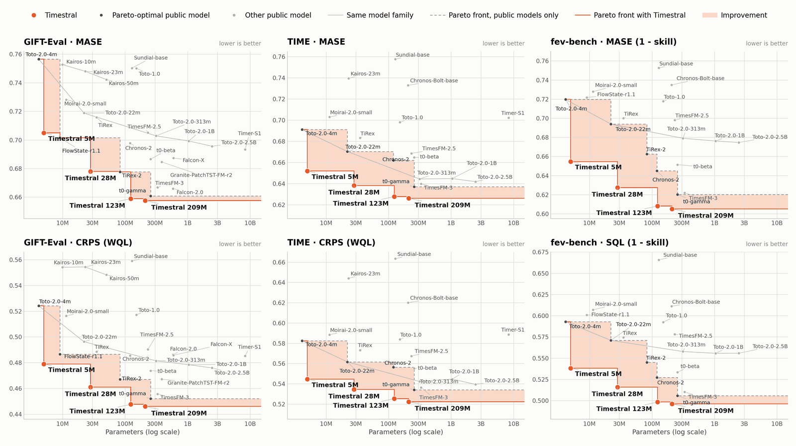
The family plot is the more interesting claim. The 28M model scores 0.678 MASE on GIFT-Eval, against Chronos-2's 0.698 (reported, card). The 123M is within 0.001 of the 209M on GIFT-Eval MASE, 0.659 against 0.658 (reported, card; measured in the same files). If you are choosing a size, the curve is nearly flat above 123M.
The licence is the catch
The code is Apache-2.0. The weights are not. They ship under a "Modified MIT License" whose second clause reads: "You are not authorized to exercise any rights under this license if the global consolidated monthly revenue of your company (or that of your employer) exceeds $20 million". The clause covers derivatives too, and points larger companies to Mistral's sales team or hosted services (measured, the LICENSE file in each model repository). fev-bench's model registry records Timestral as commercial_use: false.
The users the blog describes, plants with thousands of sensors and finance teams forecasting flows, are mostly companies above that line. For them Timestral is a model to evaluate, then license or rent through Mistral Forge.
What I take from it
The architecture is not exotic: patches of 32, causal scaling with an asinh squash, a gated trunk where every fourth layer looks across variates, and a quantile head that cannot cross. The new piece, forecast-token decoding, is a mask and one learned vector in code. So most of the result is in the training recipe, synthetic-first with a context grown from 8,192 to 32,768 (reported), which the coming report will have to explain.
The headline holds where I could check it: the card's GIFT-Eval and fev-bench numbers reproduce from the leaderboards' own files to the third decimal, and among public, single-checkpoint, zero-shot models it is first on both. "State of the art" needs the asterisk that one unreleased model has a lower GIFT-Eval MASE, and that agent ensembles sit above all of them.
It is also small and cheap. A 96-step probabilistic forecast from 2,048 steps of history takes about half a second on two shared CPU threads with symmetric averaging on, and from the full 32,768 steps about 6.5 s, in 1.84 GB of RAM. Running a forecaster no longer needs a GPU. Using this one commercially, above $20 million a month, needs a contract.
For more on how open model releases are assembled, see Mistral Large 4 and Leanstral; for another foundation model that forecasts from tokens, with its own calibration problems, see Kronos. Datadog's Toto family, one of the models Timestral is compared against, comes up in the Scout piece.