2026-10-10 · 28 min · finance · time-series · tokenization · autoregressive · calibration · benchmarks · pretraining
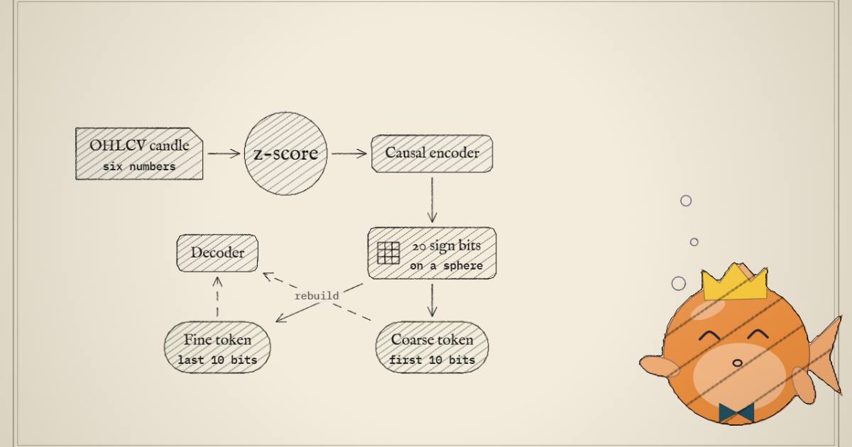
Why read this
Hightop 30%Kronos's tokenizer and sampler from the code, a real-data tokenizer widget, the headline ratios rebuilt, and 8,533 live-demo forecasts scored.
- Analysis found nowhere else
- Interactive explanations
- Runs on a laptop CPU
LLM architectureMITPractitioner model
How this was scored
- Is it new?
- 2 of 3: A real new idea, method or capability
- Can I trust it?
- 2 of 3: Measures key facts from files, code or configs
- Can I run it?
- 2 of 3: Open code or weights with real limits
- Will I understand it?
- 3 of 3: Mechanism carried by interactives built from real code or data
- Can I act on it?
- 2 of 3: A concrete recipe, numbers or comparison
- Will it last?
- 2 of 3: A reference for a year or more
- Does it affect many?
- 1 of 3: A specialist community
- Only here?
- 3 of 3: The only place this analysis exists
Score 75 of 100, ranked 54 of 494 rated articles. Each question is answered 0–3 by hand, and a 3 is rare. How articles are scored
Kronos calls itself "the first open-source foundation model for financial candlesticks". The pitch is a neat one: a candlestick chart is a language, so tokenize it and train a GPT on it. The paper (arXiv 2508.02739, accepted at AAAI 2026) reports a 93% RankIC improvement over the best time-series foundation model, and the repository links a live Bitcoin forecast that refreshes every hour.
I wanted to know two things. How do you turn an open-high-low-close-volume bar into a token without throwing away what matters? And what do those big percentages measure?
The first answer is clever and worth stealing. The second is less exciting than the abstract makes it sound. Along the way I found that the live demo has kept every forecast it ever made in its git history, 8,571 commits of them, so I scored them.
- license
- MIT
- branch
- master
- tests
- 6 files
- source
- 492.4 kB
- commit date
- 2026-04-13
by size of tracked source at this commit, file counts in brackets; docs, data and vendored trees excluded
local clone, 2026-10-10 at 67b630e — branch, commit, commitDate, fileCount, hasTests, languages, license, licenseFile, shallow, testFileCount
shallow clone: counts describe the pinned tree, not the history
A candle, before it is a token
A K-line (the Chinese and Japanese name for a candlestick) is one bar of market data: open, high, low and close prices, plus volume and "amount", the money traded. Kronos takes all six, which the paper calls OHLCVA.
The first thing KronosPredictor.predict does to them is throw away the price level. Each column is z-scored over the context window you pass in, then clipped:
# model/kronos.py:544-547
x_mean, x_std = np.mean(x, axis=0), np.std(x, axis=0)

x = (x - x_mean) / (x_std + 1e-5)
x = np.clip(x, -self.clip, self.clip)   # clip = 5
So the model never sees "10.93 yuan" or "62,000 dollars". It sees "a bit above the average of the last 512 bars, and the high is two standard deviations out". This is instance normalisation, the same move Chronos and most time-series foundation models make, and it is why one model can read Bitcoin and a Shanghai small-cap. It also means a forecast is only ever relative to the window you chose. Pass 100 bars or 500 and you are asking a different question.
If a series has no volume, predict() fills volume and amount with zeros (kronos.py:528-530). The paper says it zeroed both on 5% of training samples so the model learns to cope with that.
Time enters separately. Every bar's timestamp becomes minute, hour, weekday, day of month and month (calc_time_stamps, kronos.py:472-479), each with its own learned embedding, summed onto the token embedding (module.py:536-562). The model is told it is 09:35 on a Wednesday. It is never told which exchange or asset it is looking at.
Twenty bits per candle
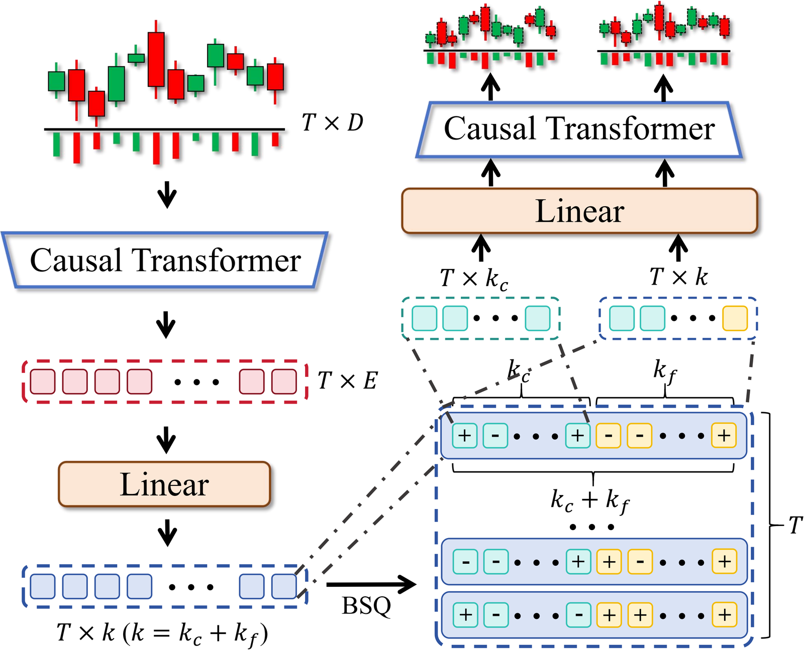
The tokenizer is a small autoencoder. A linear layer lifts the 6-vector to 256 dimensions, a few causal transformer blocks mix in the preceding bars, and a linear layer projects down to 20 numbers. Then comes the quantizer, which is the interesting part:
# model/module.py:245-247  (BSQuantizer.forward)
z = F.normalize(z, dim=-1)                       # put the 20-vector on the unit sphere
quantized, bsq_loss, metrics = self.bsq(z, collect_metrics=collect_metrics)

# model/module.py:85-88  (BinarySphericalQuantizer.quantize, constants simplified)
zhat = torch.where(z > 0, 1, -1)
return z + (zhat - z).detach()                   # straight-through estimator
That is Binary Spherical Quantization (BSQ), borrowed from video tokenizers (Zhao, Xiong and Krähenbühl). There is no codebook to look up. Every coordinate's sign is a bit, so 20 coordinates give 220 = 1,048,576 possible codes with zero codebook parameters. Normalising onto the sphere first bounds how far any input can sit from its code, which is the paper's argument for why a flash-crash bar cannot blow up the error. The bits are scaled by 1/√20 so the code is itself a unit vector.
The twist is what Kronos does with those 20 bits. The first 10 are the coarse sub-token and the last 10 the fine one. Nothing about BSQ makes the first half more important; the training loss does. The decoder is run twice, once on the coarse 10 bits alone and once on all 20, and both reconstructions are penalised:
# finetune/train_tokenizer.py:141-144
recon_loss_pre = F.mse_loss(z_pre, batch_x)   # decoded from the first 10 bits only
recon_loss_all = F.mse_loss(z, batch_x)       # decoded from all 20
recon_loss = recon_loss_pre + recon_loss_all
loss = (recon_loss + bsq_loss) / 2
The coarse half is forced to be a usable low-resolution candle on its own, and the fine half learns the residual. The paper's tokenizer ablation (Table 9) shows this costs almost nothing: reconstruction MAE 0.0785 with the hierarchical loss against 0.0781 without it.
I ran the released Kronos-Tokenizer-2k on the 512 five-minute candles bundled in the repo's tests/data/regression_input.csv (an A-share-style series from 2024-06-18 to 2024-07-03; the file does not name the ticker). Decoding from the coarse 10 bits gave a mean squared error of 0.0076 in normalised units; all 20 bits brought it to 0.0048. In price terms, over the last eight candles, the coarse code is off by 0.0135 on average and the full code by 0.0083, on a stock trading near 10.9. The fine bits buy roughly 40% less error, and the coarse bits already carry most of the candle.
The widget below is that run. Every number in it is what the tokenizer produced, not a simulation.
grey: the real candle · colour: what the decoder rebuilt from the coarse 10 bits · click a candle
| field | real | coarse | full |
|---|---|---|---|
| open | 10.900 | 10.900 | 10.889 |
| high | 10.900 | 10.913 | 10.897 |
| low | 10.830 | 10.880 | 10.862 |
| close | 10.870 | 10.894 | 10.876 |
| volume | 2,668 | 2,695 | 2,684 |
Two things in it surprised me. First, the 09:35 bar, the first of a new session after an overnight gap, has a low of 10.83 that the coarse code smooths to 10.88; the fine bits pull it back to 10.862. That is the hierarchy doing what the paper says. Second, those 512 candles used only 108 distinct coarse ids and 44 distinct fine ids out of 1,024 each. One quiet stock over two weeks lives in a small corner of the vocabulary. The paper reports that over its corpus the coarse codebook is 97.66% used and the fine one 85.25%.
One more detail from the code: the tokenizer is not a per-candle lookup. The encoder and decoder are causal transformers over the whole window, so a bar's code depends on the bars before it, and so does its reconstruction. "Tokenize a candle" really means "tokenize a candle in context". The causal mask also means a code never depends on bars after it, which matters for leakage.
Two small vocabularies instead of one big one
A 1,048,576-entry vocabulary would need a 1,048,576-row embedding table and a 1,048,576-way output head. The paper works it out for the base model in Table 12: 1,842.3M parameters with one vocabulary, of which 1,744.8M are vocabulary, against 102.3M when the code is split in two. So Kronos predicts a token in two steps, coarse first, then fine given coarse:
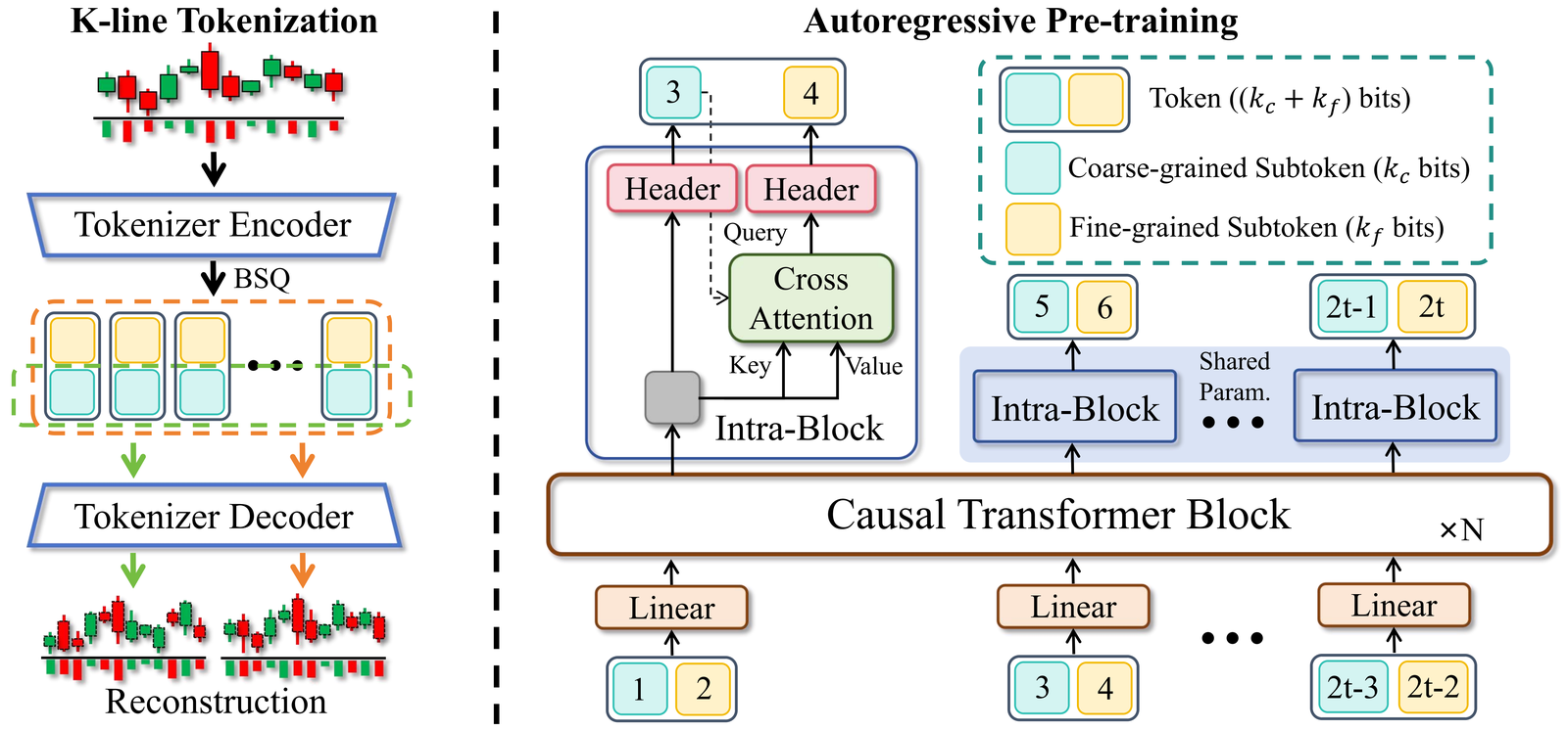
In code, the input side embeds each half in its own 1,024-row table and fuses them with one linear layer (HierarchicalEmbedding, module.py:400-443). The trunk is a plain pre-norm decoder: RMSNorm, rotary position embeddings, SwiGLU feed-forward, causal attention (module.py:465-483). The output side is where the dependency lives:
# model/kronos.py:265-276  (Kronos.forward, training path)
s1_logits = self.head(x)                       # coarse head
if use_teacher_forcing:
    sibling_embed = self.embedding.emb_s1(s1_targets)
else:
    s1_probs = F.softmax(s1_logits.detach(), dim=-1)
    sample_s1_ids = torch.multinomial(s1_probs.view(-1, self.s1_vocab_size), 1).view(s1_ids.shape)
    sibling_embed = self.embedding.emb_s1(sample_s1_ids)

x2 = self.dep_layer(x, sibling_embed, key_padding_mask=padding_mask)   # cross-attention
s2_logits = self.head.cond_forward(x2)                                 # fine head
DependencyAwareLayer (module.py:446-462) is a single cross-attention: the coarse token's embedding is the query, the trunk's hidden states are keys and values. Note the default: during training the fine head is conditioned on a coarse token sampled from the model's own prediction, not the true one. finetune/train_predictor.py:108 calls model(...) without use_teacher_forcing, so this is what actually runs. The paper says it does this to reduce exposure bias, and its ablation (Table 2) has the sequential version beating a variant that predicts both halves at once: price-series RankIC 0.0254 against 0.0226.
If this shape looks familiar, it should. MiniMax's music model does the same thing at a different scale, a global model for the first codebook and a local one for the rest. It is the standard answer to "my tokenizer has a huge implicit vocabulary".
What was released
The README lists four models. Three are on Hugging Face under NeoQuasar, all MIT. I read the safetensors headers with HTTP range requests and summed every tensor:
| Checkpoint | Layers | d_model | Heads | Context | Parameters (from headers) |
|---|---|---|---|---|---|
| Kronos-mini | 4 | 256 | 4 | 2048 | 4,108,192 |
| Kronos-small | 8 | 512 | 8 | 512 | 24,741,696 |
| Kronos-base | 12 | 832 | 16 | 512 | 102,311,008 |
| Kronos-large | 18 | 1664 | 32 | 512 | not released (paper: 499.2M) |
| Kronos-Tokenizer-base / -2k | 3 + 3 | 256 | 4 | n/a | 3,958,234 each |
The README's 4.1M, 24.7M and 102.3M are exact. Two small things the configs show. The tokenizers' config.json says n_enc_layers: 4, but KronosTokenizer.__init__ builds range(self.enc_layers - 1) blocks (kronos.py:60-68), so there are 3 encoder and 3 decoder blocks, matching the paper's text. And Kronos-mini is not in the paper at all; it is a later release with its own tokenizer, trained for a 2,048-bar context. The large model, the one that tops every table, is the one you cannot download.
- task
- time-series-forecasting
- license
- mit
- safetensors
- 1 shard
- largest file
- 409.3 MB
- files
- 4
- downloads
- 726.5K
- likes
- 286
repo last modified 2025-09-09
- task
- time-series-forecasting
- license
- mit
- safetensors
- 1 shard
- largest file
- 99.0 MB
- files
- 4
- downloads
- 1.0M
- likes
- 34
repo last modified 2025-09-09
- task
- time-series-forecasting
- license
- mit
- safetensors
- 1 shard
- largest file
- 16.4 MB
- files
- 4
- downloads
- 423.3K
- likes
- 33
repo last modified 2025-09-09
- task
- time-series-forecasting
- library
- pytorch
- license
- mit
- safetensors
- 1 shard
- largest file
- 15.8 MB
- files
- 4
- downloads
- 2.3M
- likes
- 81
repo last modified 2025-09-09
- task
- time-series-forecasting
- library
- torch
- license
- mit
- safetensors
- 1 shard
- largest file
- 15.8 MB
- files
- 4
- downloads
- 409.5K
- likes
- 11
repo last modified 2025-09-09
Twelve billion candles, mostly from four places
The pretraining corpus is the paper's Table 13. I summed it: 12,105,393,655 observations across 96,569 instruments, matching the table's own "12.11B" total. The 45 exchanges are real, but the weight is not spread evenly. NASDAQ, NYSE, Shanghai and Shenzhen together are 68.8% of all candles, mostly because they are the only stock venues with 1-minute bars and history back to 2000 (the US) or 1990 (China). Binance adds another 10.2%. Everything in China, counting futures and indices, comes to 31.9%. Of the 47 exchange rows, 39 start in 2020 and 27 carry only daily and weekly bars.
The cleaning pipeline (Appendix B) splits series at large open-to-previous-close jumps, which removes splits and contract rolls, cuts out runs of zero-volume or frozen-price bars, and drops segments shorter than a per-frequency minimum. Crypto, futures and forex are up-weighted during training.
What I could not check: the data is not released, and the paper does not say whether delisted instruments are included. "8,725 assets" on NASDAQ since 2000 is the kind of count you would expect with dead tickers in it, but that is a guess. Survivorship matters less for a model that only ever sees a normalised window of one series than for a backtest, but it still shapes what "typical" looks like. The paper puts the end of the pretraining data at June 2024 and starts every test in July 2024.
Sampling, and what predict() throws away
Forecasting is ordinary autoregressive decoding with one oddity per step. auto_regressive_inference (kronos.py:389-469) encodes the context into coarse and fine ids, then for each future step runs the trunk, samples a coarse id with temperature and top-p, runs the cross-attention with that id, samples a fine id, and appends both. Past max_context it rolls the buffer. At the end it decodes the whole window back to six numbers per bar through the tokenizer's decoder and un-normalises.
You can ask for many paths with sample_count. Here is what happens to them:
# model/kronos.py:465-467
z = z.reshape(-1, sample_count, z.size(1), z.size(2))
preds = z.cpu().numpy()
preds = np.mean(preds, axis=1)
The paths are averaged before you ever see them. The README calls this "probabilistic forecasting", and the docstring of predict_batch says the samples are "automatically averaged internally", which is accurate. The paper's Figure 7 shows why they did it: averaging more paths raises IC and RankIC, from about 0.020 RankIC on price series with one path to 0.0265 with twenty.
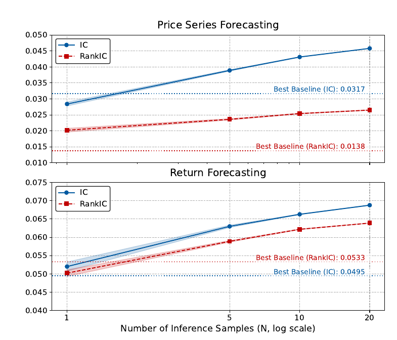
Read the bottom panel closely: with one sample, return-forecasting RankIC is about 0.050, below Moirai's 0.0533. The lead over the baselines needs the ensemble. That is a fair thing for a sampler to do, but it means the "single model" in the comparison is really a ten-path average (Table 6 sets N = 10 for forecasting, at T = 0.6).
What you lose by averaging is the spread, which is the whole point of sampling a financial series. If you want the fan, the cheapest route with the shipped code is to pass the same series N times to predict_batch with sample_count=1:
paths = predictor.predict_batch(
    [x_df] * 20, [x_ts] * 20, [y_ts] * 20,
    pred_len=24, T=1.0, top_p=0.9, sample_count=1, verbose=False)
closes = np.stack([p["close"].values for p in paths])   # (20, 24)
That is what I did, once, with Kronos-mini on CPU: 512 bars of context, 24 steps, 20 paths. It took 24.1 seconds on two threads and peaked at 769 MB of RAM. Toggle the widget to "real run" to see it. The context sat in a narrow range, the paths spread to between 10.84 and 11.09, and the price that followed ended at 11.05, which 3 of the 20 paths reached or passed. One run on one series that sits right at the pretraining cutoff proves nothing about skill, and I am showing it only so the fan has real data in it. The toy tab lets you move N and temperature and watch the median, the 10–90% band and the "share ending higher" settle.
predict() hands backWatch the last box as you drag N. With 30 paths the "probability of going up" can only move in steps of 3.3 points, and its stability depends on how correlated the paths are. Hold that thought for the demo.
What a RankIC of 0.0267 means
The abstract's headline numbers are ratios: "boosts price series forecasting RankIC by 93% over the leading TSFM and 87% over the best non-pre-trained baseline". I rebuilt both from the appendix tables. Averaged across 11 markets, Kronos-large's price-series RankIC is 0.0267. The best zero-shot foundation model is Time-MoE base at 0.0138, and the best trained-from-scratch model is TimesNet at 0.0143. 0.0267 over 0.0138 is 1.93; over 0.0143 it is 1.87. The arithmetic holds.
What is being correlated is the part the abstract does not say. An IC, information coefficient, is a Pearson correlation between forecast and outcome; a RankIC is the same on ranks (Spearman):
In quant equity work the default meaning is cross-sectional: each day, rank all stocks by predicted return, rank them by realised return, correlate, then average over days. That is the number a long-short book lives on. Appendix D defines "price series forecasting" differently: "For each sample, the IC and RankIC are calculated between the predicted and true series for each of the four price channels", then averaged. It is a correlation across the forecast horizon of one path, say 96 five-minute steps. It asks whether the predicted path goes up and down in the same order as the real one, which mostly rewards getting the drift direction right. It is a reasonable diagnostic. It is not the cross-sectional RankIC a reader with a finance background will assume.
The "return forecasting" task is closer to the usual meaning: one predicted return per sample, correlated across all samples within an asset class and frequency. That pools across time and across assets, so it is still not a per-day cross-section. There Kronos-large reaches 0.0675 RankIC against Moirai base's 0.0533 and DLinear's 0.0423. Still ahead, by a smaller margin than the headline.
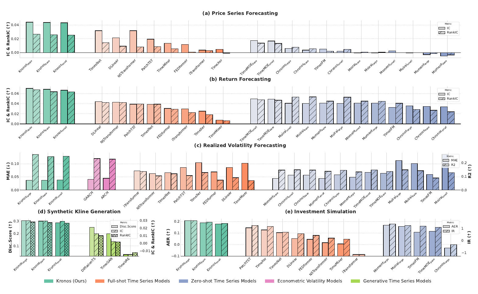
Small correlations are normal in markets, and they can matter. A daily cross-sectional RankIC that holds steady around a few hundredths, over hundreds of names and hundreds of days, is the kind of signal practitioners trade on. They can also mislead in three ways that all apply here. A percentage gain on a tiny base is easy to make large: 93% is 0.0129 of correlation. The day-to-day noise of a correlation over a few hundred items is far bigger than its mean, so you need many independent periods before the mean means anything. And the zero-shot baselines scoring around zero on price series (Moirai's three sizes average 0.0000, 0.0009 and 0.0005; TimesFM 0.0021) tells you this metric is hard for models that predict a smooth mean path, which may say as much about the metric as the models.
The lab below is a toy cross-section of 300 invented stocks. Set the built-in skill to 0.03, look at how many days come out negative, then see how many days it takes for the t-statistic to clear 2.
one bar per day: Spearman correlation of forecast and outcome across 300 names (axis ±0.25); dashed: the mean
On the baselines. The paper compares against TimesFM (without a size or version), Moirai small, base and large, Chronos small, base and large, Moment and Time-MoE, all zero-shot. It does not include Chronos-Bolt, public since late 2024, or the newer TimesFM 2.5. The trained-from-scratch baselines (iTransformer, PatchTST, TimesNet and friends) were given an MSE-plus-IC loss and 12 epochs with early stopping, which is a fair effort. None of the foundation models were fine-tuned, and neither was Kronos.
Volatility: the old model is still in the room
"A 9% lower MAE in volatility forecasting" is Kronos-large's 0.0370 against GARCH's 0.0405, the best baseline in Table 18. GARCH is from 1986. It is not just close on average: on NASDAQ it beats Kronos-large on both MAE (0.1259 against 0.1503) and R² (0.2271 against 0.0978), and on Hong Kong and Japan its R² is higher too (0.3295 against 0.1824; 0.2434 against 0.1996). Averaged R², Kronos-large leads, 0.2624 to 0.2323.
Here volatility is the realised variance of the predicted close path, one sampled path at T = 0.9. Using a generative model to sample paths and measuring their roughness is the more convincing use of Kronos to me, because it does not need the model to know which way the price goes. It needs it to know how much it wiggles, which is far more predictable.
Synthetic candles
For generation the paper trains an LSTM to tell real sequences from generated ones and reports its test error as the "discriminative score", where 0.5 would mean indistinguishable. Kronos-large averages 0.3048 against DiffusionTS's 0.2504, the "22% improvement in generative fidelity". Read it the other way and the classifier still separates real from Kronos-generated candles about 70% of the time. Better than the baselines, not yet fooling a one-layer LSTM with 32 hidden units. The train-on-synthetic, test-on-real scores (Table 21) are again small correlations: 0.0282 average RankIC for Kronos-large against 0.0102 for DiffusionTS.
The backtest
The investment simulation runs inside Microsoft's Qlib on China A-shares: each day rank the CSI 300 (or CSI 800) by the forecast 10-day average return, hold the top 50 equally weighted, swap at most 5 a day, hold at least 5 days, charge 0.15% per trade. Table 10 gives Kronos-large an annualised excess return of 0.2193 over the CSI 300 with an information ratio of 1.4177.
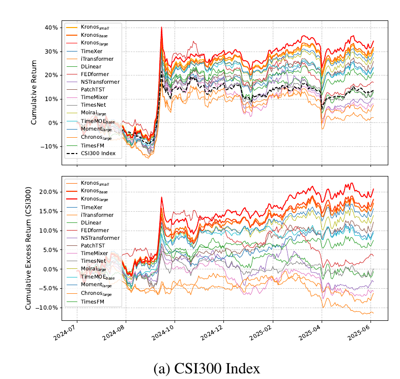
I read this chart by eye, so take the next numbers as approximate. Before the last week of September 2024, Kronos-large's excess return is a few percent. In that week, when Chinese equities rallied violently on a stimulus package, it jumps to about 18%, and so do most of the other models' excess curves. Roughly half the year's excess arrives in one week that hit everyone. Even Moment large and Moirai large, which score near zero on the price-series metric, post 0.1655 and 0.1470 annualised excess returns. When nearly every signal "beats" the benchmark by double digits, a good part of that is the setup: an equally weighted top-50 basket against a capitalisation-weighted index, over one 11-month window. The relative ordering, Kronos above the rest, is the informative part, and it rests on one period with no error bars.
The code is more careful than this makes it sound. The test windows normalise using the context only (finetune/qlib_test.py:84-87). Costs are in: open_cost 0.1%, close_cost 0.15%, a minimum of 5 per trade, fills at the next open, and a 9.5% limit threshold so you cannot buy a stock pinned at its daily limit (qlib_test.py:136-139). Qlib's TopkDropoutStrategy acts on the previous step's signal, so there is no same-day look-ahead that I can see; I am going by Qlib's convention here and did not run the backtest. There is no market-impact model, which for a 50-name CSI 300 book is a smaller omission than it would be for small caps.
One thing does differ between paper and code. The paper's signal (Eq. 13) divides the forecast move by the price. The repository's signal is the predicted close minus the last close in normalised units (qlib_test.py:276-281), so it is divided by each stock's own recent standard deviation, a volatility-scaled score. Neither is wrong; they rank stocks differently.
The repository's own figures/backtest_result_example.png comes from this fine-tuning demo, and its README carries a sober note: "A robust quantitative strategy requires more sophisticated techniques, such as portfolio optimization and risk factor neutralization." I agree with it.
Fine-tuning, two ways
The finetune/ pipeline is the Qlib one above: CSI 300 daily bars from 2011, train to 2022, validate to mid-2024, test from April 2024 to June 2025, a 90-bar lookback and 10-bar horizon (finetune/config.py:14-38). It fine-tunes the tokenizer first, then the predictor, both with torchrun. Its dataset computes the normalisation from the lookback only, with a comment saying why: "Mean and std are calculated strictly on the lookback window (past data) to prevent future data leakage" (finetune/dataset.py:107-113).
The newer finetune_csv/ pipeline, for any CSV of candles, does not:
# finetune_csv/finetune_base_model.py:120-127
window_data = self.data.iloc[start_idx:end_idx]        # lookback + predict window
x = window_data[self.feature_list].values.astype(np.float32)
x_mean, x_std = np.mean(x, axis=0), np.std(x, axis=0)  # includes the bars being predicted
x = (x - x_mean) / (x_std + 1e-5)
The mean and standard deviation include the future bars. During training, the context therefore carries a faint hint of where the target goes, and at inference predict() normalises on the context alone, so the model trains on one distribution and runs on another. It will not wreck a fine-tune, but it can make validation loss look better than live use. The example config also sets test_ratio: 0.0, so the sample Alibaba run (93,912 five-minute bars of 09988.HK from 2019-11-26 to 2025-09-17) has no held-out test set; its pictures in finetune_csv/examples/ are validation-period plots. The README warns that many comments in finetune/ were written by Gemini 2.5 Pro and "may contain inaccuracies", which is a candid thing to put in a README.
The live demo, scored
The live demo shows a 24-hour BTC/USDT forecast with an "upside probability" and a "volatility amplification" probability.
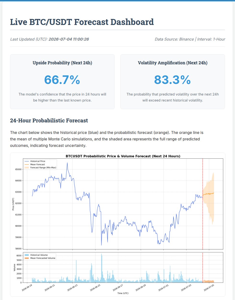
The first thing to notice is the date. On 2026-10-10 it still showed 2026-07-04. The script behind it is in the Kronos-demo repository: update_predictions.py loads Kronos-mini and Tokenizer-2k, pulls the last 384 hourly candles from Binance, drops the one still forming (df_full.iloc[:-1], so no peeking at an unfinished bar), passes the remaining 383 to the model (the page says 360; 360 is only what the chart plots), samples 30 paths at T = 1.0 and top-p 0.95, and reports the share of paths whose last close beats the last real close. It then commits the page and the chart to git, every hour. The demo also ships its own copy of kronos.py whose predict() returns every path rather than their mean, which is why it can draw a band and the main repository cannot.
Is it cherry-picked? No, and the authors deserve credit for that. Every forecast went into the repository's history automatically: 8,571 commits from 2025-07-11 to 2026-07-04. That also means it can be checked. I pulled the index.html from every commit, read the probability and its timestamp, and compared each with Binance's hourly BTC/USDT closes 24 hours later.
Over 8,533 hourly forecasts:
- BTC ended the 24 hours higher 49.5% of the time. The demo's average upside probability was 52.3%.
- The Brier score of its upside probability was 0.318. Saying "50%" every hour scores 0.25, and lower is better. The forecast was worse than a coin.
- When it said 80% or more, BTC rose 48.1% of the time (1,636 forecasts). When it said 20% or less, 46.2% (1,089). On the 398 occasions it said 100%, the price was up 51.0% of the time.
- Hourly forecasts overlap, since each looks 24 hours ahead. Taking only the 00:00 UTC forecast each day gives 355 independent-ish calls: Brier 0.328, and the direction was right on 49.7% of the 344 that were not exactly 50%.
- The rank correlation between the upside probability and the realised 24-hour return was 0.018.
- The "volatility amplification" probability scored a Brier of 0.2519 against 0.25 for always guessing the base rate of 50.6%.
None of this shows Kronos is useless. Kronos-mini is the smallest model, nobody can call one-day Bitcoin direction reliably, and the paper never claims a calibrated probability. What it shows is narrower and, I think, more useful: the fraction of 30 sampled paths that end up is not a probability. The paths share most of their drift, so they tend to agree with each other far more than they agree with the market. A dashboard that turns that fraction into "66.7% upside probability" is presenting sampler agreement as confidence. If you sample paths from Kronos for risk work, calibrate the spread against outcomes before you trust it.
Smaller things in the repository
- The README's quick-start reads
./data/XSHG_5min_600977.csv. That file is not in the repository at HEAD (67b630e, 2026-04-13), and the raw URL returns 404. The regression test data intests/data/is the usable bundled sample. tests/test_kronos_regression.pypins exact Hugging Face revisions of Kronos-small and the base tokenizer and decodes greedily (top_k=1), so the outputs are reproducible to a relative tolerance of 1e-5. That is good practice and unusual for a research repo.examples/has grown community scripts that are not the model.examples/prediction_new.pymultiplies Kronos's forecast by a hand-built "adjustment factor" from macro and sector heuristics (prediction_new.py:720-745); the JSON reports inexamples/yuce/carry hard-coded entries like a holiday-effect "historical_win_rate" of 0.8.examples/run_backtest_kronos.pyfalls back to the predicted price when the actual one is missing and charges no costs. Treat these as somebody's experiments, not Kronos results.webui/is a small Flask app that loads any of the three released sizes and plots a forecast against held-back data.
What I would use it for
Kronos is a well-made piece of engineering. The tokenizer is the part I would take away: a codebook-free quantizer with a bounded error, a training loss that gives the bits an order of importance, and a two-step head that turns a million-way softmax into two 1,024-way ones. That pattern applies anywhere a multivariate step needs to become a token, sensor frames as much as candles. The models are small, MIT-licensed and run on a laptop CPU; Kronos-mini forecast 24 steps with 20 paths in under half a minute.
As a forecaster, it is a strong baseline among foundation models on the paper's own metrics, with the caveats above: a headline metric that is a within-path correlation rather than a cross-section, a lead over baselines that needs a ten-path average, a volatility win over GARCH that is narrow and not universal, a backtest that is one window dominated by one week, and a public demo whose probabilities are uncalibrated. If you want to try it, use it as one feature among many, fine-tune with the lookback-only normalisation, and measure it on your own out-of-sample period with costs. This article is an explanation of a model, not trading advice.
For related reading on the site: the Transformer and rotary embeddings explainers cover the trunk Kronos uses; EVA is another case of an autoregressive prior over learned latents; and Interfaze 1 Lite ships TimesFM 2.5 as its forecasting component, the baseline Kronos never ran.
How I checked
- Read the paper (arXiv v1, the only version, HTML and PDF) including all appendices, and parsed Tables 13–21 from the arXiv HTML. The ratios behind 93%, 87%, 9% and 22% are recomputed from those tables. Figures 4, 7 and 9 exist only in the PDF and were rendered from it at 220 dpi.
- Shallow-cloned
shiyu-coder/Kronosat67b630eand readmodel/,finetune/,finetune_csv/,webui/,examples/andtests/; line numbers above are from that commit. - Read
config.jsonand the safetensors header of all fiveNeoQuasarKronos checkpoints with HTTP range requests and summed the tensor shapes (integer buffers excluded for the tokenizers). - Ran Kronos-mini and Kronos-Tokenizer-2k once on CPU (PyTorch 2.14.1, two threads) on
tests/data/regression_input.csv: a tokenizer round trip on the first 512 bars, then one 20-path, 24-step forecast throughpredict_batch. Wall time 38 s including model load, peak RSS 769 MB. The tokenizer widget and the "real run" tab are the recorded outputs. - Cloned
shiyu-coder/Kronos-demowith--filter=blob:none, batch-fetched theindex.htmlblob of each of its 8,571 commits, and parsed the update time, upside probability and volatility probability. Matched each to Binance BTCUSDT 1-hour closes (fromdata-api.binance.vision): last complete close at the forecast hour against the close 24 hours later. The gap between 8,571 commits and 8,533 forecasts is placeholder commits from the first day and repeated updates within the same hour, of which I kept the last. - Rendered the live demo with headless Chromium through
puppeteer-core. - Not checked: the pretraining data (not released), Kronos-large (not released), the backtest itself (needs Qlib's A-share data), and whether the published weights are the exact checkpoints behind the paper's tables.