2026-10-31 · 25 min · multi-token-prediction · pretraining · self-distillation · speculative-decoding · gradients

Why read this
Notabletop 60%Derives the gradient split, checks it in float64, then runs the authors' own tests, losses and released checkpoints on CPU; results at scale are the paper's.
- Original analysis
- Runs on a laptop CPU
- A lasting reference
Training & RLMITResearch paper
How this was scored
- Is it new?
- 2 of 3: A real new idea, method or capability
- Can I trust it?
- 2 of 3: Measures key facts from files, code or configs
- Can I run it?
- 2 of 3: Open code or weights with real limits
- Will I understand it?
- 2 of 3: Mechanism from first principles with figures
- Can I act on it?
- 2 of 3: A concrete recipe, numbers or comparison
- Will it last?
- 2 of 3: A reference for a year or more
- Does it affect many?
- 1 of 3: A specialist community
- Only here?
- 2 of 3: A teardown or measurement few others did
Score 67 of 100, ranked 207 of 666 rated articles. Each question is answered 0–3 by hand, and a 3 is rare. How articles are scored
Multi-token prediction (MTP) has become a routine ingredient of language-model pre-training: extra heads predict the tokens after the next one, the model learns from a denser signal, and the heads double as a draft model for speculative decoding. Multi-Token Prediction Done Right (Jayden Teoh, MIT; arXiv 2610.38331, submitted 2026-10-28, CC BY 4.0) argues that the standard loss has a flaw, and that the fix is a single line. The post that brought it to my attention puts it as h_ntp += h_mtp.detach() - h_mtp, "a free lunch for MTP".
A claim that a gradient identity is exact is a claim I can check, so most of this article is checking. The paper's results at 167M to 1.2B parameters are the authors' and are marked reported. What I did myself is marked measured: I rederived the decomposition, tested it in float64 on 300 random cases and in float32 on a small transformer, ran the repository's own tests, compared the authors' released 167M checkpoints (same tensors, and the effective rank of the output head), and timed the cost of the alternative. I also trained a toy model, with limits spelled out in its own section.
Correction, 2026-10-31. The first version of this article said I had not run any of the repository's code and that every number on the method came from my own reimplementation. That was true then and is not now. I have since cloned the repository (commit 4e1cf66), run its test suite (17 of 17 pass on CPU), trained its own model class and its own four losses at toy scale, and loaded its released 167M checkpoints into its own model class. One thing I wrote before running it turned out wrong: my toy said Soft-MTP gives the best draft agreement, and the authors' own model code does not reproduce that at 300 steps. The details are in What running their code showed; the toy section below is kept as it was, with its claim now labelled as one implementation's result.
The setup, and what "position-aligned" means
A language model maps a prefix to a hidden state and a linear output head (a matrix, shared by every head below) turns it into a distribution over the next token: . The next-token loss is the cross-entropy against the actual next token .
MTP adds extra heads. Head at position produces its own hidden state and predicts the token steps further on, , through the same matrix . (Two designs exist: parallel heads, as in Gloeckle et al., and the sequential DeepSeek style where each head also consumes the embedding of the token it just skipped. The analysis does not depend on which.) The total loss is the next-token loss plus an average of the extra cross-entropies, weighted by .
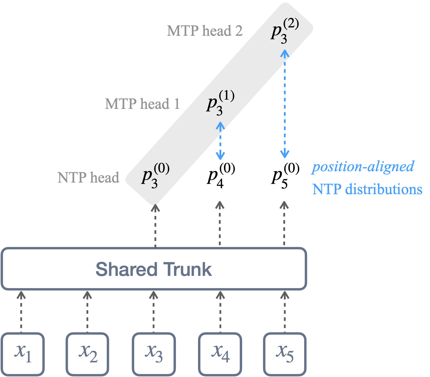
The observation that everything follows from is in the paper's Figure 2. The token that head predicts at position is also the token that the ordinary next-token head predicts at position . So for every MTP prediction there is a position-aligned NTP distribution, , aimed at the same target by the same model.
Splitting the gradient
Back-propagating the cross-entropy of head to its hidden state gives a familiar vector. With the head's distribution and the one-hot target,
Add and subtract the aligned NTP distribution :
This is an identity, nothing more. But both pieces mean something. The first is exactly the gradient, with respect to the head's hidden state, of the KL divergence from a stop-gradient copy of to : a pull of the MTP head toward the model's own next-token distribution. That is self-distillation, and it is what makes the draft heads agree with the verifier in speculative decoding. The second is the cross-entropy gradient that the aligned NTP hidden state would receive for the same token. It depends on which token was sampled.
The card below does the arithmetic for one position over a five-word vocabulary. Draw targets from the teacher's distribution and watch the two pieces: the KL piece does not change with the draw; the residual does, and on average it is bigger.
The expected squared length of the residual, when the sampled token follows the teacher's distribution, is : a floor set by the teacher's entropy that training the head cannot lower. The KL piece shrinks as the head catches up with the teacher. The paper's argument for removing the residual is a bias-variance one. Splitting into , with the true distribution of the next token, gives an "NTP error" term that shrinks as the model improves and a one-hot sampling-noise term with mean zero that never does. Dropping the residual removes the noise at the price of a bias toward the NTP distribution instead of the data, a trade that gets better with scale and one the paper argues is the right one for a head whose job is to match its verifier.
The trick: put the missing gradient where it can be found
To keep and drop , you need to subtract at the MTP hidden state. The paper's observation is that already exists in the computation: it is the gradient the aligned NTP hidden state receives from its own cross-entropy. So route it.
Replace the NTP hidden state at position with
The bracket is exactly zero in the forward pass, so the NTP logits, the NTP loss and the gradient reaching are unchanged. In the backward pass the bracket is not zero: the NTP cross-entropy's gradient at is , and it flows into with a minus sign. Add the head's own cross-entropy gradient and
No teacher is cached, no second softmax is formed, and the loss value reported is the ordinary hard loss. In the repository's implementation the line carries a scale factor, ntp_hidden[:, head:] = ntp_hidden[:, head:] + kl_recovery_scale * (head_hidden.detach() - head_hidden), which accounts for the mean over NTP positions, the mean over the positions of head , and the weighting (loss.py, line 174 of commit 4e1cf66; the factor is derived in the paper's Appendix B.5).
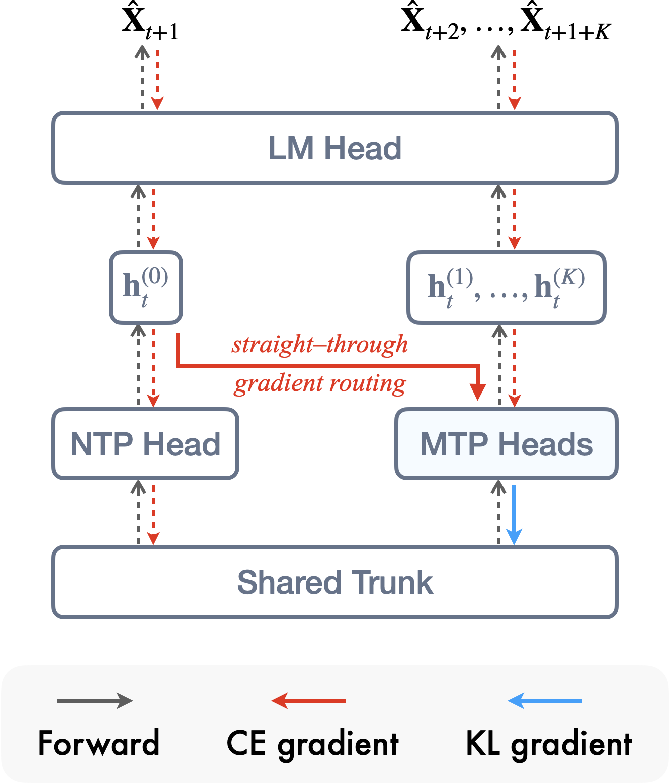
There is one subtlety the paper states and the diagram below makes concrete. The trick recovers the KL gradient for everything upstream of the MTP hidden states: the MTP heads and the shared trunk. The shared output head still receives the ordinary cross-entropy gradient from both the NTP and the MTP losses. An explicit KL objective would instead send a KL gradient into too. The paper argues the difference is a feature, and shows an effect of it at 1.2B that I will come back to.
What I checked
The identity, in float64 (measured). I built random instances of the setup: a shared output head and hidden states for positions and MTP heads, treated as free variables, with vocabulary size from 8 to 399, width from 4 to 63, from 6 to 39, from 1 to 4 and from 0.25 to 1.75. Over 300 such instances, using PyTorch's autograd on the augmented loss:
- The augmented NTP loss equals the plain one exactly: the largest difference is 0.0.
- The gradient with respect to the NTP hidden states is identical to the unaugmented one, again 0.0.
- The gradient of the augmented-NTP-plus-MTP loss with respect to every MTP hidden state matches the gradient of the explicit KL, computed by autograd, to a largest absolute difference of , a largest relative difference of (float64 rounding), and the closed form to the same level.
- The decomposition holds to .
- With the repository's normalisation (means instead of sums, the weighting and the per-head scale), the gradient equals to .
Through a trunk (measured). To see parameters rather than hidden states, I gave each of 40 instances a tiny trunk and heads and compared the Soft-MTP gradient with that of an explicit objective that is cross-entropy for the next token plus times the KL for each head. Trunk and head gradients agree to . They differ from plain MTP's by up to 0.26 (gradient scale about 0.56). The shared output head behaves as the paper's gradient-routing table says: Soft-MTP's gradient equals plain MTP's exactly (difference 0.0) and differs from the explicit-KL objective's by 0.085.
On a real (small) model, in float32 (measured). I repeated the comparison on the toy transformer used further down (537,856 parameters, a 2,048-token vocabulary, two trunk layers, three sequential MTP heads), on one batch. Soft-MTP's trunk gradient matches the explicit KL objective's to a worst relative difference of and its MTP-head gradients to , float32 round-off; it differs from plain MTP's trunk gradient by 57%. The output-head gradient equals plain MTP's (0.0) and differs from the explicit-KL objective's by 61%. The reported loss is bit-identical to plain MTP's.
The authors' own gate (measured). The repository's tests/test_kl_recovery.py checks the same four things in float64: head and trunk gradients of soft_mtp equal those of direct_kl; the two differ only at the shared unembedding; the head gradient equals the closed form; and the forward value is untouched because the coupling is x.detach() - x. My check was written from the paper before I read it, so the two are independent confirmations. The first version only read this file. I have now run it: pytest tests -v on commit 4e1cf66 with torch 2.14.1 and transformers 5.20.2, CPU, gives 17 passed in 7.8 s (log: public/articles/soft-mtp/verify/pytest.out). That includes the mutation check, which perturbs the recovery scale by 0.5 and 2.0 and confirms the identity then fails, so the gate can fail. The repository is MIT-licensed; the paper is CC BY 4.0.
The released checkpoints (measured). The authors published NTP, standard-MTP and Soft-MTP models at 167M, 332M, 689M and 1.2B parameters (twelve repositories under JaydenTeoh/; the 689M one declares an MIT licence). The 167M hard-MTP and Soft-MTP files have the same 366 tensors and 178,368,512 parameters (the NTP-only model has 327 tensors and 167,154,176): "adds no parameters" holds, and the MTP heads cost 11.2M parameters, 6.7% of the base model.
The paper's Figure 6 reports that standard MTP collapses the effective rank of the readout (the unembedding multiplied by the final RMSNorm gain, effective rank in the sense of Roy and Vetterli) and that Soft-MTP stays closest to the NTP baseline: 496 for NTP, 131 for standard MTP, 321 for KL-MTP and 437 for Soft-MTP at 1.2B. I fetched only the unembedding and norm tensors of the three 167M models by byte range and computed the same quantity:
| 167M model | effective rank of the logit map (of at most 512) |
|---|---|
| next-token only | 468.3 |
| standard MTP | 436.4 |
| Soft-MTP | 464.5 |
The ordering matches the paper, and at this scale the collapse is mild (7% below the baseline for standard MTP, against 74% at 1.2B in the paper). That fits the paper's claim that the problem grows with scale, though it is one training run per model and says nothing about cause.
The cost (measured). The paper's Table 5 reports, at 1.2B on a single H200 GPU, that Soft-MTP is within 0.07% of standard MTP's throughput while explicit KL costs 1.5% more FLOPs, 5.6% throughput and 21 GB of peak memory. I have no GPU here, but the mechanism is visible on a CPU. For one step of the combined loss at 512 tokens, width 512, a 50,304-token vocabulary and three heads, averaged over two runs (CPU seconds, peak resident memory):
| objective | CPU seconds per step | peak memory |
|---|---|---|
| standard MTP | 4.81 | 1.14 GB |
| Soft-MTP | 5.08 (+5.5%) | 1.04 to 1.19 GB |
| explicit KL | 7.05 (+46%) | 1.51 GB (+32%) |
The Soft-MTP difference is within the run-to-run spread on this loaded machine (the two runs differ by 0.3 s); the explicit KL's extra cost is not. The extra time and memory come from materialising a teacher and a student distribution over the vocabulary for every head, which the trick never does and which standard fused cross-entropy kernels avoid by design.
A toy run, and where it disagrees
To see the objectives behave rather than only their gradients, I trained a toy model on a CPU: a 537,856-parameter transformer (two trunk layers, width 64) with three DeepSeek-style sequential MTP heads, a 2,048-entry BPE vocabulary trained on three public-domain books (542,232 tokens, a tenth held out), 300 steps, , three seeds per objective with the same seeds across objectives so the comparisons are paired. Four objectives: next-token only; standard MTP; explicit KL (KL gradient at the heads, trunk and the shared output head); and Soft-MTP with the repository's scale factor. This is far from the paper's setting, and "toy" is the right word: the held-out loss ends near 5.6 nats per token (a perplexity of about 270; a uniform guess is 7.6), so the next-token teacher is poor. All numbers below are measured, from public/articles/soft-mtp/code/results.jsonl.
| mean over 3 seeds (± standard deviation) | next-token only | standard MTP | explicit KL | Soft-MTP |
|---|---|---|---|---|
| held-out next-token loss, nats | 5.610 ± 0.019 | 5.542 ± 0.015 | 5.609 ± 0.017 | 5.661 ± 0.020 |
| extra-head cross-entropy | n/a | 5.382 | 5.686 | 5.722 |
| KL from the next-token distribution to the heads | n/a | 0.182 | 0.071 | 0.062 |
| top-token agreement with the next-token head | n/a | 0.596 | 0.725 | 0.736 |
| expected accepted draft length (teacher-forced) | n/a | 2.20 | 2.64 | 2.68 |
What agrees with the paper (in my own toy implementation; the authors' own code, tested in the next section, does not agree at this training length):
- The drafts get better. Soft-MTP's heads agree with the next-token head's top choice far more often than standard MTP's (0.736 against 0.596, higher in all three seeds), sit closer to its distribution (KL 0.062 against 0.182, lower in all three), and would be accepted for longer drafts (2.68 against 2.20 tokens per round, higher in all three). That is the quantity speculative decoding depends on, and it is the paper's Table 2 effect at a different scale.
- Soft-MTP and explicit KL behave alike on the drafts. The paper says they should, since they send the same gradient through the heads and trunk. Soft-MTP is slightly closer in KL in all three seeds (0.062 against 0.071) and ahead in agreement and accepted length in two of three.
- The gradient noise ordering. For the seed-0 models I measured the gradient signal-to-noise ratio of the KL component and the residual with respect to the trunk parameters (40 batches, the unbiased estimator the paper cites). The KL component has the higher ratio in both: 2.07 against 0.34 on the standard-MTP model and 0.43 against 0.15 on the Soft-MTP model. The residual's gradient norm is 1.23 and 0.97 times the hard gradient's, the KL part's 0.67 and 0.21 (norm ratios can exceed 1 because the two components partly cancel). The paper reports about 4× lower signal-to-noise for the residual and about 80% of the trunk gradient at 167M to 1.2B; mine is one model of each kind at a tiny scale, so it supports the ordering and nothing about the size.
What does not:
- The loss gain. Standard MTP beats the next-token-only baseline on held-out next-token loss (5.542 against 5.610, in all three seeds), the usual MTP benefit. Soft-MTP is worse than standard MTP by 0.119 (all three seeds) and worse than the next-token-only baseline by 0.050 (all three seeds). The paper reports the opposite at every scale it trained, 167M and up. My model is a few hundred times smaller and trained for a few hundred steps, so this does not contradict the paper; it is a different regime.
A reading of why, which I have not tested further: in the paper's own bias-variance argument, the residual is the sum of the teacher's error and sampling noise, and Soft-MTP removes both. Early in training, or in a very small model, the teacher's error is large and carries real information about the data that the next-token head has not yet learned; dropping it costs the trunk a useful signal, while the noise it removes matters less. The paper argues the trade turns favourable as the teacher improves. I did not train longer or larger models to check, so treat this as a hypothesis that fits the direction of the evidence.
What running their code showed
The toy above is my own transformer. The repository ships its own model class (HFMTPForCausalLM: RoPE, RMSNorm, SwiGLU, sequential DeepSeek-style heads with per-head final norms) and its own four losses (ntp, hard_mtp, soft_mtp, direct_kl in src/models/loss.py). All numbers here are measured, on CPU, with torch 2.14.1 and transformers 5.20.2. I skimmed the entry points first for network, subprocess and pickle use, and ran only the tests, the model and loss modules, and my own loops around them.
The line. The stop-gradient trick is one statement, loss.py line 174 at commit 4e1cf66: ntp_hidden[:, head:] = ntp_hidden[:, head:] + kl_recovery_scale * (head_hidden.detach() - head_hidden). It runs inside the same loop that computes the plain cross-entropy for each head, and direct_kl is a separate function that materialises the teacher softmax.
Their tests. 17 of 17 pass, as above. That settles the identity for the real implementation, not only for my reimplementation of it.
Their model and losses, trained small. I built a 615,680-parameter instance (width 64, two trunk layers, three sequential heads, a 2,048-entry vocabulary), took the same tokens and the same AdamW schedule as my toy, and trained each objective for 300 steps with three seeds, calling the repository's model(input_ids, labels=…) so that its loss code does the work. Same corpus and held-out split as before; the architecture is theirs, so the numbers differ from the toy table.
| 300 steps, mean over 3 seeds | next-token only | standard MTP | explicit KL | Soft-MTP |
|---|---|---|---|---|
| held-out next-token loss, nats | 4.872 | 4.933 | 4.926 | 5.022 |
| KL from the next-token distribution to the heads | n/a | 0.045 | 0.081 | 0.078 |
| top-token agreement with the next-token head | n/a | 0.773 | 0.652 | 0.654 |
| expected accepted draft length | n/a | 2.84 | 2.36 | 2.37 |
Two results differ from my toy and one holds.
- Contradicted: the draft-agreement gain, at 300 steps. In my toy Soft-MTP agreed with the next-token head more than plain MTP (0.736 against 0.596). In the authors' own model code, at the same 300 steps, plain MTP agrees more (0.773 against 0.654, higher in all three seeds) and sits closer in KL (0.045 against 0.078, all three seeds). Explicit KL and Soft-MTP are indistinguishable from each other, which is what the identity predicts for the heads. So the statement in the first version of this article that my toy "reproduces the draft-agreement gain" was a property of my toy and of 300 steps, not of the method.
- Not what I expected: the gain appears with more training. I retrained plain MTP and Soft-MTP with the authors' code for 1,500 steps (two seeds, not three, to fit the machine). Now Soft-MTP agrees more (0.733 against 0.700, both seeds), is closer in KL (0.106 against 0.139, both seeds) and has the longer accepted draft (2.67 against 2.55). That is the paper's direction, reached once the next-token head is a less poor teacher. I did not train further, so I do not know where it settles.
- Confirmed: the loss is worse. Soft-MTP's next-token loss is above plain MTP's at 300 steps (5.022 against 4.933, all three seeds) and at 1,500 (4.169 against 4.105, both seeds), and above the next-token-only baseline at 300 steps. In this model plain MTP does not beat next-token only either (4.933 against 4.872), unlike in my toy. The paper's loss gain is a claim about 167M parameters and up; nothing I ran at 0.6M parameters speaks for it.
Cost, on a loaded machine with two jobs sharing the CPU: 0.13 s per step for next-token only, 0.24 for plain MTP, 0.23 for Soft-MTP and 0.35 for explicit KL, so Soft-MTP matched plain MTP and explicit KL cost about half as much again, in line with the cost table above.
The released checkpoints, run. Earlier I only read tensors out of the released 167M files. This time I loaded all three (next-token only, plain MTP, Soft-MTP) into the repository's own model class, with no missing or unexpected keys, and measured them on 12,288 positions of the three public-domain books (they were trained on FineWeb-Edu, so these are out-of-domain; the books are Austen, Shelley and Doyle).
| 167M checkpoint | next-token loss | top-token agreement, heads 1 to 3 | KL to the next-token head, heads 1 to 3 | accepted length |
|---|---|---|---|---|
| next-token only | 3.280 | n/a | n/a | n/a |
| plain MTP | 3.338 | 0.689, 0.636, 0.611 | 0.339, 0.473, 0.560 | 2.39 |
| Soft-MTP | 3.325 | 0.703, 0.650, 0.623 | 0.327, 0.454, 0.533 | 2.45 |
This is one checkpoint per objective, so no variance is available, and the books are not the paper's test set. The direction is the paper's: Soft-MTP's heads agree more and sit closer in KL at every head, its next-token loss is lower than plain MTP's, and the next-token-only model has the lowest loss on this text. The gaps are small, as they are in the paper at this size. Parameter counts (178,368,512 for both MTP models, 167,154,176 for next-token only) match the tensor listing above.
Not run. Training at the paper's scale (FineWeb-Edu, Muon, 167M and up) and the lm_eval and speculative-decoding evaluation need a GPU and days; I ran none of it.
Scripts, logs and raw results are in public/articles/soft-mtp/verify/.
What the paper reports
All of this section is reported, from the paper's own tables; I did not rerun any of it. The setup is LLaMA-style models from 167M to 1.2B parameters, DeepSeek-style sequential MTP with three extra heads, trained on about 31.5B tokens of FineWeb-Edu with the Muon optimizer, .
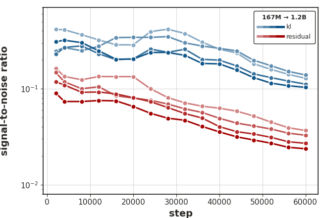
- Why the residual hurts. Measured over 256 batches, the residual's gradient signal-to-noise ratio is about 4× lower than the KL component's (4.1× at 167M, 4.6× at 1.2B), yet it carries about 80% of the MTP gradient that reaches the shared trunk. A step along it in the trunk's hidden state raises the NTP loss, a step along the KL component lowers it.
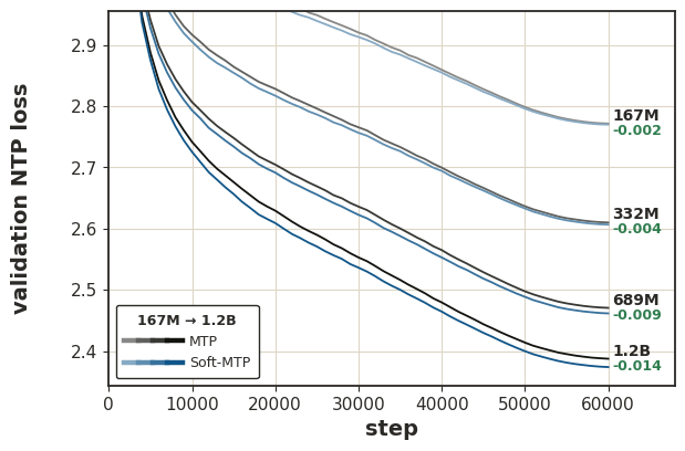
- Pre-training loss. Soft-MTP ends below standard MTP on next-token validation loss at every scale, by 0.002 (167M), 0.004 (332M), 0.009 (689M) and 0.014 (1.2B), read from the labels of the paper's Figure 4; from 689M it is also lower on the MTP loss.
- Speculative decoding. The MTP heads used as drafts agree slightly better with the verifier. At 167M the self-speculative speedup on FineWeb-Edu goes from 1.90× to 1.92× and the mean accepted length from 1.52 to 1.54, and the KL to the verifier from 0.485 to 0.470; at 332M the speedup goes from 1.96× to 1.98× and the KL from 0.448 to 0.430.
- Downstream accuracy. Zero-shot average accuracy is higher than standard MTP at every scale, by about 0.1 points at 167M and 332M and about 0.5 at 689M and 1.2B, where Soft-MTP also exceeds the NTP baseline.
- Fine-tuning at 1.2B (MTP heads discarded, NTP loss only): HumanEval pass@64 is 39.02 for NTP, 40.85 for standard MTP and 43.90 for Soft-MTP; MBPP pass@64 is 58.80, 59.80 and 61.00; GSM8K 47.69, 48.60 and 49.66; MATH-500 24.80, 23.20 and 25.00. Soft-MTP leads standard MTP in seven of the eight cells and is the only objective that never falls below the NTP baseline.
- Against explicit KL at 1.2B (Table 6): Soft-MTP ties or wins every perplexity metric (FineWeb-Edu 10.74 for both, WikiText 17.49 against 17.53, LAMBADA 14.07 against 14.30), has the higher average accuracy (57.31 against 57.22) and the higher code scores, while explicit KL leads on math fine-tuning. The paper attributes the remaining gap to keeping cross-entropy at the shared head: a KL objective, it argues, can be reduced by "making the shared readout less sensitive" to the directions in which MTP and NTP hidden states differ. That is its explanation for KL-MTP's lower readout rank (321, against 437 for Soft-MTP and 496 for NTP at 1.2B, Figure 6).
What I would be careful about
- The identity is exact; the benefit is empirical. Everything in the first half of this article is algebra and checks to machine precision. Whether the residual's noise actually hurts, and by how much, is a statement about trained models, and the evidence for it at 167M to 1.2B is the paper's. My own training toy cannot speak to scale.
- A bias is traded for a variance. Without the residual, the MTP heads are pulled toward the NTP distribution, not the data. The paper says so (Section 5.3) and argues it is desirable for drafts. If you want MTP heads that improve the main model's own predictions in ways its next-token head does not capture, a bias toward that head is not obviously what you want.
- It needs a shared output head. The trick, as derived, relies on the MTP and NTP positions being read out through one matrix. Architectures with separate heads have no such identity.
- Two MTP designs, limited coverage. The paper tests DeepSeek-style heads at all scales and Meta-style parallel heads at 332M. Beyond that, it varies the MTP weight (0.25 to 1.0) and the horizon (3 to 8) only at 332M, in its Figure 5.
- Small runs disagree on loss, and on agreement early. In my 300-step toy and in the authors' own code at the same size, Soft-MTP has the worst next-token loss of the MTP variants. Its draft-agreement advantage appeared in my toy at 300 steps, but with the authors' model only after 1,500. The paper's setting is different enough that this is not a refutation, but it is a reminder that both benefits are claims about models that are already good.
- The gap is small at small scale. At 167M the paper's own numbers are about +1% speculative-decoding speedup and 0.002 in loss. The argument that it grows with scale rests on four model sizes, and I found no mention of seeds or confidence intervals in the paper.
Sources
- Jayden Teoh, Multi-Token Prediction Done Right, arXiv 2610.38331 (CC BY 4.0). Figures 1 to 4 above are the paper's own.
- Code and checkpoints: JaydenTeoh/Soft-MTP (MIT; commit
4e1cf66, 2026-10-30), models under huggingface.co/JaydenTeoh. - The announcement post by @jayden_teoh_.
- On this site: the FastMTP quant analysis, for what multi-token prediction heads look like as speculative-decoding drafts in a shipped model.
- Scripts for every measurement above are in
public/articles/soft-mtp/code/(my reimplementation) andpublic/articles/soft-mtp/verify/(runs of the authors' code: tests, training, released checkpoints).
- license
- MIT
- branch
- main
- tests
- 1 file
- source
- 182.6 kB
- commit date
- 2026-10-30
by size of tracked source at this commit, file counts in brackets; docs, data and vendored trees excluded
local clone, 2026-10-31 at 4e1cf66 — branch, commit, commitDate, fileCount, hasTests, languages, license, licenseFile, shallow, testFileCount
shallow clone: counts describe the pinned tree, not the history