2026-09-19 · 29 min · explainer · llm · training · alignment · rlhf
The version of ORPO that travels is four sentences long. Why run SFT and RLHF as two stages? ORPO merges them. It penalises the rejected response directly during SFT, with no reference model. Massive compute and VRAM savings from a single objective.
The middle two sentences are exactly right. The last one is the only claim in the set with a magnitude in it, and it is the only one nobody has attached a number to. This piece attaches one — and derives the objective properly on the way, because the interesting part of ORPO is not that it removes a stage (plenty of methods do) but which ratio it contrasts with, and why. That is an argument about gradients, the paper makes it carefully, and almost nobody repeats it.
Short version of where this lands. The odds ratio is a genuinely good idea and the derivation rewards reading. The reference-model saving is real, and it is about 11% of model-state memory and 25% of per-step arithmetic — and it is absent entirely in the one setup where it would have mattered most. And ORPO's best result is in a table the paper never printed.
The premise: SFT teaches the rejected response too
Everything follows from one observation in §3. Cross-entropy on the chosen response raises the probability of the chosen tokens and says nothing at all about the rejected ones — the label indicator is zero for every non-answer token, so there is no term in the loss that pushes anything down. What actually happens, empirically, is that fine-tuning on chosen-only data drags the rejected responses up alongside them, because the two share a style, a domain and most of their vocabulary.
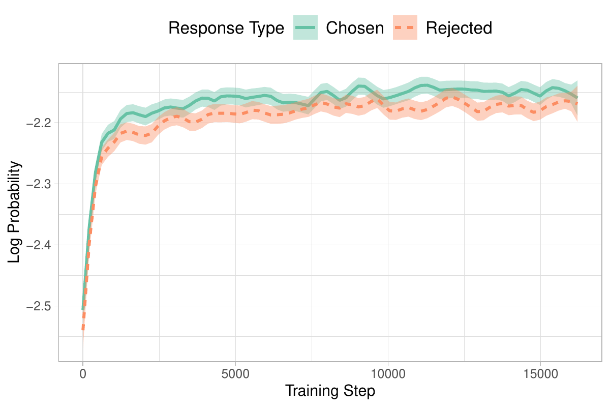
Read the axis before you accept the claim. The whole chart spans 0.35 nats, the two curves separate by roughly 0.02 nats at convergence, and the ribbons overlap for most of the run. The paper's own summary — "the absence of a penalty for unwanted generations results in rejected responses sometimes having even higher log probabilities than the chosen ones" — is stronger than this figure supports for this model; after step 2000 the chosen curve is above the rejected one throughout. What the figure does show cleanly is the thing that matters: the rejected curve goes up, by about the same amount as the chosen one, and nothing in the SFT objective was ever going to stop it.
So the fix is not exotic. Add a term that pushes the rejected response down. The interesting question is which term.
The objective, in five lines
Start with the quantity the whole method is built on. ORPO's is not the joint probability of the sequence. Equation 3 defines it through an average:
which makes the geometric mean of the per-token probabilities:
This is load-bearing and it is the detail most summaries drop. Hold onto it; in two sections it will be the only thing keeping the odds ratio from collapsing into the probability ratio.
Now the odds of generating , and the ratio of two of them:
Wrap the log of that in a log-sigmoid so that minimising it means increasing the log odds ratio, and you have the penalty term:
Add it to the ordinary negative log-likelihood with a weight, and that is the entire method:
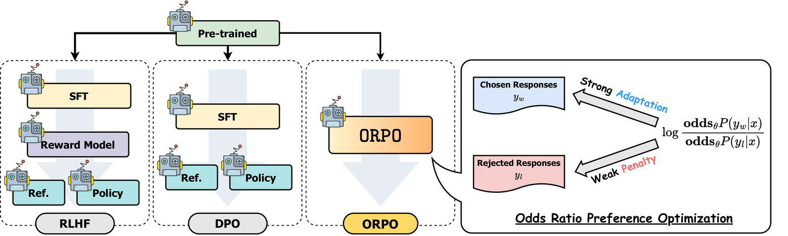
Two things are worth noticing about that objective before moving on. First, the SFT term never leaves — ORPO is not a replacement for supervised fine-tuning, it is supervised fine-tuning with a second term bolted on, which is why the paper calls it monolithic rather than reference-free alignment. Second, there is no anywhere. DPO's objective is built from the ratio , so it structurally requires a second set of weights; ORPO's is built only from evaluated on two sequences.
Why an odds ratio and not a probability ratio
This is the part of the paper that earns it. §7.1 asks the obvious question — DPO and IPO contrast a probability ratio, so why not
— and answers it with a distributional argument. Since the log-sigmoid is what the ratio gets fed into, what matters is the scale of the thing going in. A loss of the form is small when is a few units positive; how hard the optimiser has to push to get there depends entirely on how wide 's natural range is.
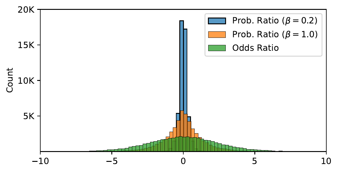
The paper makes this point with 50,000 Monte Carlo samples and leaves it qualitative. It has an exact answer, and the exact answer is nicer. For , is , so is standard Laplace with standard deviation ; and is standard logistic with variance , so the difference of two of them has standard deviation . That gives:
| quantity | exact sd | sd, 400k samples | fraction within ±1 |
|---|---|---|---|
| , | 0.2828 | 0.2832 | 99.3% |
| , | 1.4142 | 1.4158 | 63.1% |
2.5651 | 2.5678 | 32.3% |
(My arithmetic and my simulation, reproducing the paper's Figure 6 setup.) The odds ratio is 1.81× wider than the probability ratio at and 9.07× wider at — and 0.1 to 0.2 is the range these methods actually run at; the ORPO paper set DPO's to 0.1 for every one of its own comparisons.
Why that matters, concretely. Hold both formulations to the same length-normalised — which is what the paper's own ablation does — fix the chosen response at a geometric-mean per-token probability of 0.6, and ask how far the rejected response has to fall before each loss is satisfied:
| target | required log-margin | odds ratio needs | prob. ratio | prob. ratio |
|---|---|---|---|---|
| 0.5 | 0.433 | 0.493 | 0.389 | 0.069 |
| 0.1 | 2.252 | 0.136 | 0.063 | 7.7e-6 |
| 0.01 | 4.600 | 0.0149 | 0.0060 | 6.2e-11 |
(My arithmetic.) To get the loss down to 0.01, the odds-ratio version needs the
rejected response's average token probability to reach about 1.5%. The
probability-ratio version at needs it to reach 6.2e-11. That is
not a penalty, it is an erasure — and erasing the rejected response is
catastrophic when you are simultaneously doing domain adaptation from a base
checkpoint, because the rejected response is still mostly fluent English in the
target domain. The paper's Appendix B shows exactly this: trained with the
probability ratio, the rejected log-probabilities crash below −4 early; with the
odds ratio the same thing only happens after overfitting sets in.
The gradient, and where the penalty actually bites
The paper gives the gradient as a product of two factors (Eq. 8–10), which is the clearest way to see what the term does:
is a gate: near 1 when the model prefers the rejected response, near 0 once it prefers the chosen one by a comfortable margin. is a contrast of the two per-sequence gradients, each divided by its own . The division is not decoration — it falls out of the algebra, because exactly, which is how Appendix A's Eq. 32 becomes Eq. 33.
Here is what those two factors do when you multiply them out. The quantity to watch is the coefficient the loss puts on — how hard it pulls the rejected response down, as a function of how likely the model currently thinks the rejected response is.
Log vertical axis, four decades. The curve that matters is the thick one: the coefficient this loss puts on ∇ log P(y_l), which is the gate δ = 1/(1+OR) times the 1/(1−P_l) amplifier from h(d). It runs from 0.0357 when the rejected response is already unlikely to 8.57 when the model prefers it — a factor of 240. That asymmetry is the whole design: on a pair the model already has right, the penalty term contributes essentially nothing and the plain SFT term runs the show; on a pair the model has backwards, the penalty dominates. “Weak penalty, strong adaptation” is not a slogan about magnitudes, it is a statement about which examples get penalised. Curves computed from the paper's Eq. 7 and Eq. 9–10 with the chosen side pinned at 0.6; moving that pin slides the curves sideways without changing the shape.
The shape is the argument. When the model already assigns the rejected response a low probability, the gate is nearly shut and the whole term contributes about 0.036 — the SFT loss runs the batch unopposed. When the model prefers the rejected response, the coefficient reaches 8.57, a factor of 240 higher. "Weak penalty, strong adaptation" turns out not to be a claim about the size of the penalty but about which examples get one. On a pair the model already has right, ORPO is just SFT.
That also explains the ablation in Appendix E, which is the paper's most useful and least quoted result. At the rejected log-probabilities do not fall at all — the chosen ones simply rise to satisfy the term. At both fall while the margin widens, and MT-Bench gets worse at extraction, math and reasoning while getting better at STEM, humanities and roleplay. The authors say so plainly: a bigger margin means "overly adapting to the chosen responses set in the training dataset". The knob that makes the LLM-judged benchmark go up makes the hard-answer categories go down.
The reference model, priced
Here is the claim worth checking, because it is the one the tweet version rests on. §7.3 argues two savings: memory, because there is no frozen resident; and compute, because "in theory, two forward passes should be calculated for each model… four forward passes happen in total for a single batch" while ORPO needs "half the number of forward passes".
The paper gives no GiB and no tokens per second. So:
The thing ORPO deletes is one frozen bf16 copy of the weights. For Mistral-7B — 7,241,732,096 parameters, the model the paper actually trained — that copy is 13.49 GiB against 107.91 GiB of trainable state, so removing it saves 11.1% of model-state memory, not 50%. My arithmetic, standard mixed-precision AdamW accounting.
| resident tensor | B / param | GiB @ 7.24B | who pays |
|---|---|---|---|
| policy weights (bf16) | 2 | 13.49 | both |
| policy gradients (bf16) | 2 | 13.49 | both |
| fp32 master weights | 4 | 26.98 | both |
| AdamW first moment | 4 | 26.98 | both |
| AdamW second moment | 4 | 26.98 | both |
| — trainable subtotal | 16 | 107.91 | both |
| frozen reference π_ref (bf16) | 2 | 13.49 | DPO only |
| — DPO total | 18 | 121.40 | DPO |
| — ORPO total | 16 | 107.91 | ORPO |
This is model state only, and it is the optimistic case for ORPO. Under LoRA the picture inverts — the trainable state is ~0.6 GiB, so a second frozen copy would nearly double memory — except that TRL's DPOTrainer keeps no second copy for a PEFT model: it disables the adapter and reuses the base weights as the reference. The saving is largest exactly where DPO does not pay it.
Thirteen and a half gibibytes, against 107.91 of trainable state. 11.1% of
model-state memory. The reference model is cheap for the same reason it is
convenient: it is frozen, so it carries bf16 weights and nothing else — no
gradients, no fp32 master copy, no Adam moments, and no stored activations,
because its forward runs under no_grad. The expensive copy of the model is the
one you are training, and ORPO still has that.
The compute claim needs the same treatment:
The paper's claim is that ORPO needs “half the number of forward passes” per batch — two instead of four — and that is exactly right. But two of DPO's four forwards are the reference model's, and those run under no_grad: they have no backward to pay for. The work that survives is the policy's four passes, two forward and two backward, and those are identical in both methods. Halving the forwards removes a quarter of the arithmetic. The independently measured number is close to this: SimPO, which is reference-free in the same structural way, reports roughly 20% less wall-clock and about 10% less peak memory against a vanilla DPO implementation on 8×H100 — the gap between 25% and 20% being optimizer and communication work that does not shrink.
Counting forwards counts the cheap third of the work. Both methods run the policy forward and backward over the chosen and the rejected sequence; DPO adds two backward-free forwards. 12P against 16P is a 25% saving. The closest thing to an independent measurement comes from SimPO, which is reference-free in exactly the same structural way and reports "roughly 20%" less run time and "about 10%" less GPU memory against a vanilla DPO implementation on 8×H100 — which lines up with the arithmetic above almost exactly.
And then there is the part that the word vanilla is carrying. From TRL's
DPOTrainer source, the reference model is not instantiated at all in two
common cases:
# Reference model
if ref_model is None:
    if is_peft_model(self.model) or args.precompute_ref_log_probs:
        # If PEFT is used, the reference model is not needed since the adapter
        # can be disabled to revert to the initial model. If precompute_ref_log_probs
        # is True, the reference model does not need to be kept in memory during training.
        self.ref_model = None
Under LoRA, DPO recovers the reference by switching the adapter off — the base
weights are . With precompute_ref_log_probs=True, the
reference logprobs are computed once in a pass over the dataset and cached as
scalars, and per-step cost drops to ORPO's. SimPO's own footnote concedes the
point: "DPO can be as memory efficient as SimPO if it were implemented to
separate the forward passes of the reference model from the actual preference
optimization. However, this implementation is not standard practice."
This is the honest shape of the saving. Full fine-tuning at 7B in bf16: ORPO saves 11% of memory and 25% of step FLOPs, and that is worth having. Under LoRA — where the second copy would have nearly doubled resident memory, since the trainable state is about 0.6 GiB against 13.49 for the frozen base — DPO already does not pay it. The saving is smallest where memory is abundant and absent where memory is tight.
The stage it genuinely removes
There is a real win underneath the overstated one, and it is operational rather than arithmetic. SFT→DPO is two training runs, two sets of hyperparameters, an intermediate checkpoint to store and choose, and a second chance to get the learning rate wrong. ORPO is one run. If you have ever explained to someone why the DPO job reads its reference weights from a directory produced by a job that finished last Tuesday, that is the saving.
Except: count the epochs. Appendix C says ORPO was "trained for 10 epochs" with best-checkpoint selection by eval loss for the OPT series, Phi-2 and Llama-2, against a baseline of one epoch of SFT plus three epochs of DPO. In the units above that is 10 × 12P = 120P against 6P + 3 × 16P = 54P — the Llama-2 headline result used roughly 2.2× the arithmetic of the pipeline it is compared against. (My arithmetic, from the paper's stated epoch counts.) Mistral is conspicuously absent from that sentence and Figure 1's caption says "a single epoch", which would make it 12P against 54P and a 4.5× saving in the other direction. Both are in the same paper. "One stage" and "less compute" are separate claims and only one of them is structural.
The results, and their denominators
The roster, so the numbers have somewhere to sit. Controlled experiments: OPT at 125M, 350M and 1.3B, four methods each, on Anthropic HH-RLHF and on binarised UltraFeedback, judged by a 1.3B reward model. Headline experiments: Phi-2 (2.7B) at , Llama-2 (7B) at , and Mistral (7B) at , all trained on UltraFeedback alone and scored on AlpacaEval 1.0 and 2.0, with MT-Bench and IFEval for the two Mistral checkpoints. Phi-2 + ORPO reaches 71.80% and 6.35%, against Phi-2 + SFT + DPO at 50.63% and 0.78% — the only matched SFT→DPO comparison above 1.3B anywhere in the paper, and a convincing one.
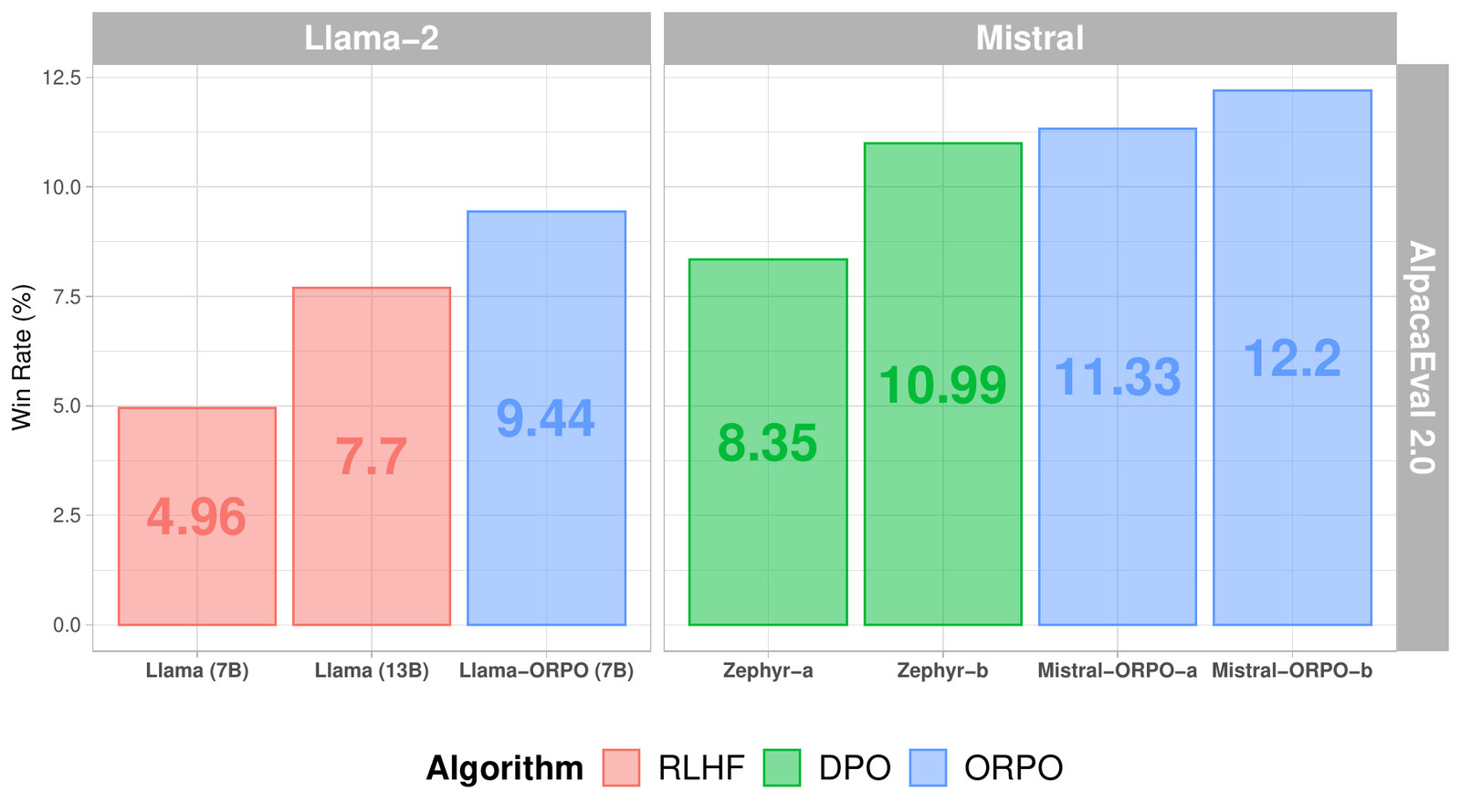
The 7B numbers are the ones that travelled, so start with what they are measured against. Every non-ORPO bar in that chart is an entry someone else put on a leaderboard. The controlled comparison at 7B did not survive: "Llama-2 + SFT and Llama-2 + SFT + DPO yielded models with outputs that could not be evaluated." Publishing that sentence is to the authors' credit and it also means the 7B column has no matched DPO baseline in it at all.
Pulled from the leaderboard's own committed data rather than from the paper, so both rows come from one evaluator run:
On the official AlpacaEval 2.0 leaderboard, Mistral-ORPO-β beats Zephyr-β by 1.57 raw points and 1.51 length-controlled points. The denominator is 805 instructions, and the margin is 17 extra head-to-head wins. Both models' standard errors are about ±1.0, so the gap is roughly one standard error — real, and not separable from noise on this benchmark alone.
| model | alignment | raw WR % | ± SE | LC WR % | wins / 805 | avg len |
|---|---|---|---|---|---|---|
| mistral-orpo-beta (7B) | ORPO, one stage | 12.57 | 0.99 | 14.72 | 95 | 1636 |
| zephyr-7b-beta (7B) | SFT → DPO | 10.99 | 0.96 | 13.20 | 78 | 1444 |
| zephyr-7b-alpha (7B) | SFT → DPO | 8.35 | 0.87 | 10.29 | 59 | 1302 |
| Mistral-7B-Instruct-v0.2 | Mistral's own post-training | 14.72 | 1.08 | 17.11 | 113 | 1676 |
Judge is GPT-4-turbo; the opponent whose outputs you must beat is also GPT-4-turbo. n_total is 805 for every row. avg_length is characters of the model's response, and it is the reason the length-controlled column exists.
Mistral-ORPO-β beats Zephyr-β by 1.57 raw points, which is 17 extra head-to-head wins out of 805 — 95 against 78. The standard errors are ±0.99 and ±0.96, so the gap is about 1.1 standard errors of itself: real, directionally consistent, and not separable from noise on this benchmark alone.
Two things the paper could not have known and one it could. Length-controlled win
rate arrived after publication, and ORPO survives it: 14.72 against 13.20,
a 1.51-point gap against the raw 1.57, so the advantage is not verbosity even
though ORPO's responses average 1636 characters to Zephyr's 1444. Good. On the
other hand Mistral-7B-Instruct-v0.2 — the instruct model Mistral shipped, with
no published preference recipe and vastly more data — sits above both at 17.11 LC.
That does not make the algorithm comparison wrong, but it is the number anyone
deciding what to actually deploy should see.
And the one it could have known: on MT-Bench, the ORPO model's own card prints Zephyr-β at 7.34 against Mistral-ORPO-β's 7.32. The abstract headlines 7.32 as an achievement; on the paper's main DPO comparator the method loses by 0.02, which is noise, and the honest word is "matches". IFEval is the clean win — 66.19% instruction-level loose against Zephyr-β's 57.67% — although the authors' own repository table shows Mixtral-8×7B-Instruct at 68.23% on that column.
The controlled experiment, read carefully
The comparison that was matched is the OPT series, 125M to 1.3B, all four methods on the same data, judged by a 1.3B reward model. Win rate of ORPO over each baseline:
| ORPO vs | 125M | 350M | 1.3B |
|---|---|---|---|
| SFT (HH-RLHF) | 84.0 | 82.7 | 78.0 |
| PPO (HH-RLHF) | 66.1 | 79.4 | 65.9 |
| DPO (HH-RLHF) | 41.7 | 49.4 | 70.9 |
| SFT (UltraFeedback) | 73.2 | 80.5 | 69.4 |
| PPO (UltraFeedback) | 71.4 | 85.8 | 65.7 |
| DPO (UltraFeedback) | 48.8 | 50.5 | 57.8 |
Against SFT-only and against PPO, ORPO wins decisively everywhere. Against DPO, below 1B, it is 41.7, 49.4, 48.8 and 50.5 — one loss and three coin flips — and it wins at 1.3B. The paper's framing, "the win rate over DPO was correlated to the model's size", is a three-point trend in each dataset and is offered as the reason to believe the 7B results. It is a reasonable hope. It is not a measurement.
Two caveats the authors supply themselves, which is worth saying because a less careful paper would not have: the judge RM-1.3B was trained on the same datasets the models were tuned on, and PPO was optimised against RM-350M and then scored by RM-1.3B — "the instability and reward mismatch problem of RLHF", in their words. The PPO column is measuring a reward-model mismatch as much as an algorithm.
That pattern repeats often enough to be worth naming. §6.4 measures lexical diversity against DPO and prints a column ORPO loses: per-input cosine similarity, where lower means more varied, comes out 0.8909 for Phi-2 + ORPO against 0.8012 for Phi-2 + SFT + DPO, and 0.9008 against 0.8889 on Llama-2. ORPO produces less varied output for a given prompt, in both families. The authors read it as ORPO "assigns high probabilities to the desired tokens" — which is a fair reading and also exactly what you would expect from a loss whose SFT term never turns off — and then publish the number either way. Together with the Llama-2 baseline that failed to produce evaluable output and Appendix E's finding that the knob trades math for chattiness, that is three results reported against the paper's own interest, which is more than most.
Where ORPO sits among the reference-free crowd
ORPO was not the first method to drop , and it landed in the middle of a cluster. Stripped to their essentials:
- CPO — SFT NLL plus . The probability-ratio version of the same idea, un-normalised for length. This is precisely the design §7.1 argues against, which makes it the most interesting neighbour.
- SimPO — . Length-normalised like ORPO, but with a target margin and no SFT term.
- KTO — still reference-dependent, but learns from unpaired thumbs-up/thumbs-down data, which is a different data-collection problem rather than a different optimiser.
- DPO — reference-dependent, the incumbent, and the thing everyone is trying to beat.
SimPO's Table 4 is the only matched comparison that includes ORPO — every objective trained on the same data from the same checkpoints, each with its hyperparameters tuned:
The only matched head-to-head that includes ORPO is the SimPO paper's, which trained every objective on the same data from the same checkpoints and tuned each one's hyperparameters. AlpacaEval 2.0 length-controlled win rate, four settings. ORPO loses to DPO in three of four and ties in the fourth.
| objective | ref model | Mistral-Base | Mistral-Inst | Llama-3-Base | Llama-3-Inst |
|---|---|---|---|---|---|
| SFT only | — | 8.4 | 17.1 | 6.2 | 26.0 |
| DPO | yes | 15.1 | 26.8 | 18.2 | 40.3 |
| IPO | yes | 11.8 | 20.3 | 14.4 | 35.6 |
| KTO | yes | 13.1 | 24.5 | 14.2 | 33.1 |
| R-DPO | yes | 17.4 | 27.3 | 17.6 | 41.1 |
| CPO | no | 9.8 | 23.8 | 10.8 | 28.9 |
| ORPO | no | 14.7 | 24.5 | 12.2 | 28.5 |
| SimPO | no | 21.5 | 32.1 | 22.0 | 44.7 |
Not my measurement, and SimPO is an interested party: it is the paper proposing the winning row. The value here is that every column was produced by one group under one protocol, which is not true of the ORPO paper's own 7B comparisons.
ORPO loses to DPO on length-controlled win rate in three of four settings and essentially ties in the fourth (14.7 against 15.1). It loses to SimPO everywhere, which is SimPO's paper, so read it with that in mind.
The head-to-head §7.1 predicted — odds ratio against probability ratio, since CPO is otherwise the same shape — comes out only half in ORPO's favour. On length-controlled win rate ORPO leads CPO in three settings of four and trails by 0.4 in the last. On Arena-Hard the same pairs split two apiece: ORPO 7.0 against 6.9 and 10.8 against 5.8, CPO 22.6 against 20.8 and 28.8 against 25.8. A theoretical argument about gradient scale predicting a 3–1 and a 2–2 is weak support, not none.
The footnote is the sharp bit. SimPO ran ORPO from the SFT checkpoint, like every other baseline, and explains why: doing so "yields better results than starting from base checkpoints." An independent group tried ORPO's headline claim — skip the SFT stage — found it worse, and put the SFT stage back. That is one reproduction, on their data, with their tuning, and it should not be the last word. It is also the single most load-bearing counter-observation in this piece.
The result the paper never reported
Which makes the next table doubly strange. It holds ORPO's best result by a distance, and it is in someone else's appendix — in the paper arguing against ORPO, no less.
The place ORPO wins is the one its own paper never measured. On the Open LLM Leaderboard tasks in SimPO's Mistral-Base setting, ORPO posts the highest GSM8K and the highest MMLU of any row — 42.15 against the SFT checkpoint's 28.13, and 63.20 against 60.10 — while DPO takes GSM8K down to 21.76 and loses 1.6 points of MMLU.
| objective | MMLU | ARC | HellaSwag | TruthfulQA | Winograd | GSM8K | avg |
|---|---|---|---|---|---|---|---|
| SFT (start point) | 60.10 | 58.28 | 80.76 | 40.35 | 76.40 | 28.13 | 57.34 |
| RRHF | 57.41 | 52.13 | 80.16 | 43.73 | 76.64 | 4.78 | 52.48 |
| SLiC-HF | 59.24 | 55.38 | 81.15 | 48.36 | 77.35 | 33.74 | 59.20 |
| DPO | 58.48 | 61.26 | 83.59 | 53.06 | 76.80 | 21.76 | 59.16 |
| IPO | 60.23 | 60.84 | 83.30 | 45.44 | 77.58 | 27.14 | 59.09 |
| CPO | 59.39 | 57.00 | 80.75 | 47.07 | 76.48 | 33.06 | 58.96 |
| KTO | 60.90 | 62.37 | 84.88 | 56.60 | 77.27 | 38.51 | 63.42 |
| ORPO | 63.20 | 61.01 | 84.09 | 47.91 | 78.61 | 42.15 | 62.83 |
| R-DPO | 59.58 | 61.35 | 84.29 | 46.12 | 76.56 | 18.12 | 57.67 |
| SimPO | 59.21 | 62.63 | 83.60 | 50.68 | 77.27 | 22.21 | 59.27 |
This is one setting. ORPO is not uniformly best across the four settings in that table — see the GSM8K deltas below. Few-shot counts are the leaderboard's: MMLU 5-shot, ARC 25-shot, HellaSwag 10-shot, TruthfulQA 0-shot, Winograd 5-shot, GSM8K 5-shot. These are multiple-choice and exact-match tasks rather than LLM-judged preference, which is why they are worth more than the win rates above, and why it is strange that the ORPO paper reports none of them.
In that setting ORPO takes GSM8K from 28.13 to 42.15, the highest in the table, while DPO takes it down to 21.76. It also posts the highest MMLU of any row, 63.20, above the SFT model it began from, in a column where DPO loses 1.6 points.
One setting is not a finding, so here is the same subtraction across all four of SimPO's settings — each objective's GSM8K minus the SFT checkpoint it was trained from:
Across all four of SimPO's settings, ORPO has the best mean GSM8K change of any preference objective: +2.50 points against its own SFT starting checkpoint, where DPO loses 8.27 and SimPO loses 10.98. Every objective with a positive mean — ORPO, SLiC-HF, CPO — carries a supervised fine-tuning term, and every objective without one is negative. The converse does not hold: RRHF has an SFT term too and sits fifth, sunk by a single catastrophic −23.35 on Mistral-Base.
| objective | SFT term | Mistral-Base | Mistral-Inst | Llama-3-Base | Llama-3-Inst | mean Δ |
|---|---|---|---|---|---|---|
| ORPO | yes | +14.02 | −3.64 | +3.72 | −4.10 | +2.50 |
| SLiC-HF | yes | +5.61 | −0.84 | +2.50 | −2.12 | +1.29 |
| CPO | yes | +4.93 | −1.75 | +0.61 | −1.29 | +0.62 |
| KTO | no | +10.38 | −1.67 | −7.35 | −11.68 | −2.58 |
| RRHF | yes | −23.35 | −2.73 | −2.04 | −2.58 | −7.68 |
| DPO | no | −6.37 | −0.16 | −7.65 | −18.88 | −8.27 |
| IPO | no | −0.99 | −1.07 | −23.65 | −10.46 | −9.04 |
| SimPO | no | −5.92 | −5.24 | −14.78 | −17.97 | −10.98 |
| R-DPO | no | −10.01 | −3.49 | −7.05 | −24.79 | −11.34 |
This corrects SimPO's own summary sentence, which reads "except for ORPO, almost all approaches lead to consistent drops in one or more settings." ORPO does drop in both Instruct settings, by 3.64 and 4.10. What is true is that its drops are small and its gains are the largest — and that the objectives clustered at the top are the ones with an SFT term, which is ORPO's design argument rather than ORPO specifically.
ORPO is first, by 1.2 points over the next row and by more than ten over DPO. And the grouping is the interesting part: every objective with a positive mean carries an SFT term, and every objective without one is negative. (The converse fails — RRHF has an SFT term and sits fifth, sunk by a single catastrophic −23.35 on Mistral-Base and otherwise mid-pack.) SimPO's own explanation is the obvious one: "except for ORPO, almost all approaches lead to consistent drops in one or more settings. We hypothesize that ORPO retains performance largely due to its supervised fine-tuning loss for regulation."
Their sentence is slightly too kind — ORPO does drop in both Instruct settings, by 3.64 and 4.10 — but the mechanism they name is right, and the grouping in the table is the evidence for it. Which makes the strongest case for ORPO nearly the opposite of the case the paper makes. The selling point is not that it deletes a stage; it is that keeping the SFT term inside the preference objective, live on every step, stops preference training from eating the model's arithmetic. Alignment tax paid in GSM8K points is a well-known cost of DPO. ORPO mostly does not pay it — and the paper reports AlpacaEval, MT-Bench and IFEval, all three LLM-judged or instruction-format, and not one multiple-choice or exact-match task that would have shown this.
In the library
ORPO is in TRL, and where it is in TRL is itself the adoption story:
from trl.experimental.orpo import ORPOConfig, ORPOTrainerNot trl.trainer. ORPOTrainer sits in the experimental namespace, whose
stability contract reads: "Anything under trl.experimental may change or be
removed in any release (including patch versions) without prior deprecation. Do
not rely on these APIs for production workloads." CPO and KTO are in there with
it. That is not a verdict on the method, but it is a data point about what a
maintainer with usage telemetry thinks is load-bearing.
Five differences between the paper and the code, all checkable in the source:
The weight has three names and a tenfold gap between its defaults. The paper
calls it and uses 0.1, 0.2 and 0.25 for its three headline models. The
reference implementation calls it alpha and defaults it to 1.0. TRL calls it
beta and defaults it to 0.1 — and says so, in the config docstring:
"Parameter controlling the relative ratio loss weight in the ORPO loss. In the
paper, it is denoted by λ. In the code, it is denoted by alpha." Given
Appendix E's finding that this knob trades open-ended quality against math and
extraction, a 10× default difference between the two implementations is not
cosmetic — and the reference repo's default is the one the paper never used.
TRL's SFT term includes the prompt. From concatenated_forward:
# orpo chosen nll loss is computed over the full prompt and response
chosen_nll_loss = cross_entropy_loss(all_logits[:len_chosen], labels[:len_chosen])
The labels there are the full concatenated input with only padding masked, so the
NLL is charged on the prompt tokens as well as the completion. The odds-ratio
term is not — it uses concatenated_labels, which masks the prompt with −100.
The reference repo has a disable_prompt_loss flag for exactly this, and it is
action='store_true', so both default to including the prompt. TRL simply has no
way to turn it off.
One forward pass instead of two. The reference implementation runs
model(...) separately on the positive and negative sequences; TRL concatenates
them into one batch, "because it's faster for FSDP." Same arithmetic,
better utilisation.
The numerics needed fixing. The loss needs , and here is a
geometric mean that climbs toward 1 as the model memorises the chosen response.
The reference repo's final commit is literally Merge pull request #29 from xfactlab/add-log1p; TRL goes further with a branched implementation:
def log1mexp(x: torch.FloatTensor) -> torch.FloatTensor:
    """Numerically stable computation of log(1-exp(x))."""
    # branch at -ln 2 ~ -0.693 to avoid cancellation
    t = -0.6931471805599453
    return torch.where(x < t, torch.log1p(-torch.exp(x)), torch.log(-torch.expm1(x)))
Worth knowing what this is defending against: at large , or many epochs, and . The stable form gets you much closer to the wall before you hit it; it does not move the wall.
The "reward" in the training curves is not an odds-ratio reward, and two of
the metrics are named backwards. TRL logs
chosen_rewards = self.beta * policy_chosen_logps and the rejected counterpart,
so rewards/margins — the line the ORPO docs tell you should trend upward — is
times the probability-ratio margin of two length-normalised
log-likelihoods, not anything to do with odds. Fine as a monitoring signal;
just not the quantity being optimised. Worse, the two metrics that are:
losses, chosen_rewards, rejected_rewards, log_odds_ratio, log_odds_chosen = self.odds_ratio_loss(...)
#   ...which returns:   losses, chosen_rewards, rejected_rewards, mean(ratio), mean(log_odds)
#   where ratio = F.logsigmoid(log_odds)
The metric called log_odds_ratio is — that is,
— and the metric called log_odds_chosen is the actual log
odds ratio. If you are watching a run and want to know whether the penalty term
is doing anything, the curve you want is the one named after the wrong thing.
So: should you use it
If you are full-fine-tuning a base model on a paired preference set and you want one job instead of two, ORPO is a reasonable choice and the objective is sound. If you are LoRA-tuning, the headline saving does not exist — TRL's DPO already keeps no second copy — and DPO or SimPO score better in the only matched comparison available. If what you care about is not regressing on math and knowledge while aligning, ORPO leads that table — though SLiC-HF and CPO sit 1.2 and 1.9 points behind it and share the mechanism, so the honest recommendation is "an objective with an SFT term in it", and ORPO is the best-performing member of that family.
The thing worth taking from the paper regardless of what you train with is §7.1. "Use the odds ratio because the probability ratio over-suppresses in a length-normalised, joint-SFT setting" is a specific, falsifiable, correct argument about gradient scale, and it generalises past this method. That part is excellent.
What would change my mind
5 claims above, and what would falsify each
Removing DPO's reference model saves about 11% of model-state memory and 25% of per-step FLOPs at 7B, not 'massive' amounts.
This is arithmetic on published parameter counts, not a measurement, and it assumes bf16 mixed-precision AdamW with no offload and no reference sharding. Run ORPO and DPO on the same 7B model, same batch shape, same hardware, and report
torch.cuda.max_memory_allocatedand step time for both. If the observed memory gap exceeds ~15% or the time gap exceeds ~30%, the ledger is missing something — most likely reference-model activations that I assumed were free underno_grad, or a DPO implementation that holds the reference in fp32. ZeRO-3 offload would move the answer in the other direction and make the reference nearly free.ORPO's advantage over SFT→DPO does not survive a matched comparison.
It rests on one table from one paper — SimPO's — which is an interested party, and on the ORPO paper's own OPT results being a coin flip below 1B. Any independent matched run at 7B or above, from the same base checkpoint on the same preference set with both objectives properly tuned, settles this. If ORPO's length-controlled win rate lands at or above DPO's in two or more settings, the reading here is wrong.
ORPO does not need an SFT warm-up — the claim in its own introduction — is doubtful.
SimPO's footnote 7 is the only evidence, and it is one sentence describing a tuning decision, not an ablation. Train the same base model twice on the same preference data, once ORPO-from-base and once SFT-then-ORPO, at matched total compute, and report both. The ORPO paper's own Mistral checkpoints are from-base and score well, so the from-base recipe clearly works; the open question is whether it is ever the better of the two.
ORPO's real advantage is downstream-task retention — GSM8K above all — not preference win rates.
This is my arithmetic on one appendix table from one paper, four settings, and the ORPO rows there were trained from SFT checkpoints rather than from base. It is also not a claim about ORPO specifically: the top three rows are the three objectives with an SFT term, so the defensible version is "objectives with an SFT term retain math," and ORPO merely leads that group. Run any two of these objectives from the same checkpoint on a second preference set with GSM8K measured before and after. If ORPO's mean delta lands below CPO's or SLiC-HF's, the ordering here is noise; if a reference-dependent objective lands positive, the grouping is wrong.
The paper's Eq. 8 has a sign error: the gradient is −δ(d)·h(d).
Finite differences on a two-logit toy model, so it is easy to check and easy to overturn. Take any with differentiable in one parameter, compare the central difference against , and see which sign matches. If a v3 of the paper prints Eq. 20 starting from , this is fixed upstream and the note should go.