2026-10-06 · 20 min · explainer · robotics · vision-language-models · agents · tree-search
A vision-language model can write down a robot trajectory. Give it a few successful demonstrations as text, the 3D positions of the objects in the scene and the arm's starting pose, and it will continue the pattern: a list of end-effector poses and gripper commands, one line per waypoint. The trouble is the same trouble every one-shot generator has. Most of the time the plan is roughly right and slightly wrong. The gripper closes two centimetres beside the block, and nothing downstream can fix that, because the arm executes the list open-loop.
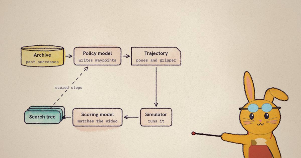
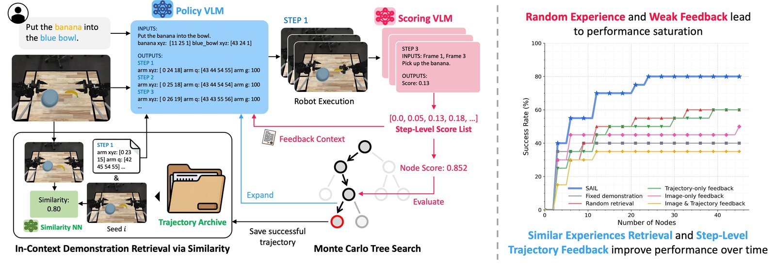
SAIL (Sakana AI and the University of Tokyo, accepted to IROS 2026) does not retrain the model to be less wrong. It runs each proposal in a simulator, has a VLM watch the video and say how far the task got, feeds those scores back as annotations on the trajectory, and asks for a rewrite. The rewrites form a tree, and Monte Carlo Tree Search decides which branch to spend the next call on. Only the trajectory that wins in simulation goes to the real arm.
The headline, from the project page:
Across six manipulation tasks in simulation, increasing the search budget from one node to 45 nodes raised the average rate of finding a successful trajectory from 25% to 73%.
That sentence is accurate. The phrase that matters is "finding". This piece walks through what a node is, how a video becomes a number, what the tree actually searches over, and then what the 25-to-73 curve does and does not measure.
What a VLM trajectory is
The paper defines the output space precisely. A trajectory for seed is a sequence of end-effector states
where is the Cartesian position, an
orientation quaternion and the gripper.
The model does not see or write floats. The state goes in as a "discretized
numeric encoding" and the trajectory comes out the same way. Figure 1 shows the
format: lines like arm xyz: [0 24 18] arm q: [43 44 54 55] arm g: 100, one per
step. An inverse-kinematics controller then drives the arm through the
waypoints in order.
The scene itself reaches the model as keypoints, not pixels in the trajectory prompt. A detection call to the same VLM marks 2D keypoints on the task-relevant objects in the overhead image, calibrated camera parameters lift them to 3D, and those coordinates plus the arm's start pose form the state . This is the lineage of Keypoint Action Tokens and "language models as zero-shot trajectory generators": the language model is a sequence model over coordinates that happens to have read a lot about bananas.
Every VLM call in the paper, for detection, generation and scoring, uses one
model: gemini-robotics-er-1.5-preview, with no fine-tuning.
Why one shot is the wrong unit
The paper's argument for search is short and correct. Trajectory space is sensitive: a small error in the predicted grasp pose is not a small error in the outcome, it is a missed grasp, and the rest of an open-loop plan then executes faithfully on nothing. A single proposal also depends on which demonstrations were in the prompt and on sampling noise. Both of those are things you can spend compute on at inference time, the way a language model spends it on sampling and checking several answers, without touching weights.
What makes this cheap enough to try is that a robot has a natural verifier that a language model usually lacks: a physics simulator. A trajectory either hands the banana from one gripper to the other in simulation or it does not. That is the part I would underline before anything else, because it is also what the headline number is measured with.
The tree: nodes are whole trajectories
SAIL's MCTS is unusual in what it puts on a node. In game-tree search a node is a state and an edge is one move. Here a node is a complete trajectory, and an edge is a rewrite of the parent trajectory into a child. Mapped onto the usual vocabulary:
| MCTS term | In SAIL |
|---|---|
| node | one complete trajectory proposal for one seed |
| edge (action) | the policy VLM rewriting the parent, given its scored annotations |
| value | the progress score of that trajectory's simulated video (next section) |
| expansion | sample refined children from the selected leaf |
| terminal | the simulator's success check passes, or the node budget runs out |
Selection walks down from the root, at each level picking the child that maximises a prior-weighted UCB (Rosin's PUCB):
is the child's mean backed-up value, a visit count, and a prior "proportional to the node's score", so a branch that scored well once is explored more. Expansion samples three children, each child is executed and scored, the scores are backed up the path, and the loop repeats until the budget is spent. Two details are easy to miss. The search stops early the moment a child passes the simulator's ground-truth success check. And each seed gets its own tree; nothing but the archive (below) is shared across seeds.
The paper does not report , the number of waypoints , or the resolution of the discretization. The budgets it runs (6, 15, 30, 45) are all multiples of three, consistent with whole expansions of children (Reasoned).
Scoring a video nobody filmed
The value of a node has to come from somewhere, and a hand-written reward per task is exactly the engineering the method is trying to avoid. SAIL uses the VLM as a progress meter, following ROVER's idea of scoring a robot video against an ordered list of subtasks.
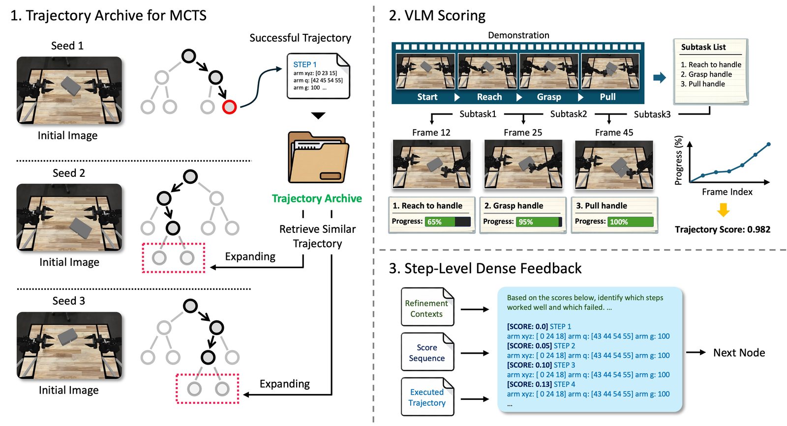
Once per task, the scoring VLM watches one demonstration video and writes the task as ordered subtasks: "reach to handle, grasp handle, pull handle" for the drawer, "grasp the blue block, move to the bowl, release the block" for the real-robot task. To score a candidate, SAIL runs it in simulation and samples frames uniformly from the video. For each sampled frame it asks the VLM one narrow question: given the current subtask, the frame where that subtask started (taken as 0%), and this frame, what percentage of the subtask is done? When the answer reaches 100%, the subtask is marked complete and the next one starts. The per-frame progress is
where is the subtask in progress at frame . The node value is the mean of over the 50 frames. A trajectory that grasps but never lifts can now beat one that misses the grasp, which a binary success signal cannot express.
The widget runs that formula on four rollouts I made up for the block-in-bowl task. The rollouts are illustrative; the arithmetic is Eq. 4.
Two properties fall out of the formula, and both are Reasoned from it rather than tested by the paper.
- The value is an area, not an endpoint. It is the mean of the progress curve, so a trajectory that finishes late scores below one that finishes early. In the widget the clean success scores 0.590 and the slow success 0.437, both passing the check. That is a reasonable bias for a robot (finish sooner) but it means a perfect trajectory does not score 1. Figure 2's example "trajectory score: 0.982" next to a rising curve would need the task to be nearly done in the first frames, so I read it as a schematic number.
- Completed subtasks are locked in. Once the VLM says a subtask hit 100%, advances and never falls below again. A block grasped and then dropped keeps its third. In the widget the "dropped in transit" rollout ends at 0.37 and scores 0.336, below the slow success but above the missed grasp's 0.174. Within one search that ordering is what you want. It also means one over-eager "100%" from the scorer is never taken back.
Each node's score costs real calls. If the scorer is queried once per sampled frame, as the method section describes, that is up to 50 scoring calls plus one generation call per node, or up to 2,295 calls for a 45-node search on one seed (Reasoned, an upper bound; early stopping cuts it).
Step-level feedback: telling the model where it went wrong
The progress curve is also the critique. SAIL aligns each sampled score to the
waypoint that was executing at that point in the video and writes the scores
into the next prompt, so the policy VLM sees its own previous trajectory as
[SCORE: 0.05] STEP 2 arm xyz: [...], with an instruction to keep the
high-scoring segments and change the low-scoring ones. The place where the score
stops rising is the place to edit.
The ablation is the strongest evidence in the paper that this matters. At a fixed 15-node budget (Reported, Table II):
| Feedback given to the policy VLM | Avg success |
|---|---|
| Step-level scores on the trajectory (SAIL) | 65% |
| Final score only | 49% |
| Previous trajectory text only | 48% |
| Rollout frames + trajectory text, no scores | 46% |
| Rollout frames only | 45% |
Showing the model its failed rollout, as images or as text, is worth no more than a single number. The scores pinned to steps are what help. On LaptopClose, step feedback reaches 50% against 30-35% for the unscored variants; on DrawerOpen and MarkerRemoveLid it is 40% each against 15% and 30% for the final score alone.
The archive: demonstrations that grow during the search
The third part is retrieval. SAIL keeps an archive of (initial image, successful trajectory) pairs, seeded with the one or few demonstrations each task starts with. Whenever the search solves a seed, that trajectory joins the archive. When expanding a node, the prompt gets the archive entries whose initial images are closest by LPIPS perceptual distance; the default is .
Again from Table II at 15 nodes (Reported): similarity retrieval with one example averages 65%; the fixed original demonstration, 45%; one random archive entry, 50%. Tripling the context to barely moves the baselines (fixed 49%, random 53%). One relevant example beats three arbitrary ones, which matches what everyone who has built a few-shot prompt has seen.
One consequence the paper does not discuss (Reasoned): the archive is shared across the 20 evaluation seeds, so a seed searched later can be handed a solved trajectory from another evaluation seed. That is legitimate for a deployed system that improves as it works. It does make the per-seed results depend on the order the seeds were run in, which the paper does not report.
The scaling curve, read carefully
Here is Table I, the result behind the headline. Each cell is the share of 20 seeds for which the search found a trajectory that passes the simulator's ground-truth check within the budget (Reported).
| Method | Nodes | Banana | Pen | Bowl | Drawer | Laptop | Marker | Avg |
|---|---|---|---|---|---|---|---|---|
| Single rollout | 1 | 40 | 40 | 40 | 10 | 15 | 5 | 25 |
| Breadth-first | 15 | 85 | 50 | 60 | 35 | 60 | 15 | 51 |
| Depth-first | 15 | 45 | 50 | 80 | 5 | 30 | 10 | 37 |
| SAIL | 6 | 80 | 55 | 100 | 20 | 50 | 25 | 55 |
| SAIL | 15 | 90 | 70 | 100 | 40 | 50 | 40 | 65 |
| SAIL | 30 | 95 | 80 | 100 | 50 | 55 | 45 | 71 |
| SAIL | 45 | 95 | 80 | 100 | 50 | 70 | 45 | 73 |
I recomputed every average from the per-task cells and all seven match the paper's rounding (Reasoned). The abstract's "up to 95%" is HandOverBanana.
Three readings follow.
The metric is "found", with an oracle. The search stops when a child passes the simulator's success check, and the table counts a seed as solved if that happened at all within the budget. So a 45-node SAIL run is being compared, in effect, against one sample, with a perfect verifier available to the larger budget. The VLM score steers the search; it is not what decides that a seed is solved. This is exactly the right design for SAIL's actual use, where the simulator is the verifier and the real robot only receives a trajectory that already passed. It is the wrong frame for reading 25% as "how good the VLM is" and 73% as "how good SAIL is" on a level field.
Most of the first jump is sampling. The fair comparison is at equal budget. Fifteen independent proposals with no feedback (breadth-first) already lift the average from 25% to 51%. SAIL at 15 nodes reaches 65%. So of the 40-point gain at 15 nodes, about 26 points come from simply trying fifteen times against the checker and about 14 from the tree, the scores and the rewrites (Reasoned). Fourteen points is real and useful. It is also the honest size of the method's contribution at that budget, and it is not uniform: breadth-first beats SAIL on LaptopClose, 60% to 50%, which the paper attributes to the fine positioning needed to pass over the screen's thin edge. Pure depth-first refinement of one chain is the worst of the three at 37%: rewriting a bad trajectory fifteen times is worse than starting over fifteen times.
The curve flattens. From 30 to 45 nodes the average moves 71% to 73%, and only LaptopClose changes. BowlOnRack is saturated at 6 nodes. DrawerOpen and MarkerRemoveLid are stuck at 50% and 45% from 30 nodes on. A tree that keeps refining the same few lineages runs out of new ideas; the paper's own Figure 1 curve is flat from roughly 24 to 45 nodes.
On noise (Reasoned): an average over six tasks is 120 seed outcomes, so a 65% average has a standard error near 4.4 points, and the 14-point gap to breadth-first is a bit over two standard errors. A single task is 20 seeds, where one seed is 5 points; per-task differences of 5 to 10 points are within what re-running would move. The paper reports no repeated runs and no error bars.
From simulator to a real SO-101
The real-robot experiment is one task: put a blue block in a red bowl with a LeRobot SO-101 arm, the same low-cost arm the FLUX 3 Action policies were adapted to. Each trial builds its own digital twin. A fixed RealSense D435i gives RGB-D; GroundingDINO finds "blue block" and "red bowl", SAM2 turns the boxes into masks, depth lifts the masks into points, an ArUco marker on the robot base gives the extrinsics, and a 3D box fit gives each object a 6-DoF pose. The simulator places its assets at those poses and matches the camera. SAIL searches in that twin with a budget of 15 nodes, stops at the first trajectory that passes, and the real arm executes it open-loop.
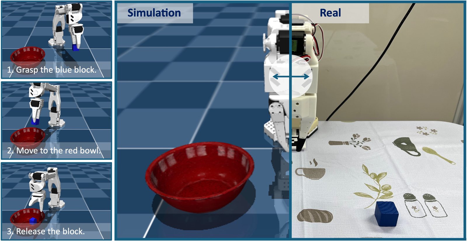
Reported: 5 of 6 real trials succeeded. The paper puts the failure on "slight errors in RGB-D pose estimation and unmodeled real-world contact dynamics". The project page's video shows six trials side by side at 2x, and its last frame agrees: in five panels the block is in the bowl, in one it sits on the cloth beside it (Measured, by looking; the page does not say which of the two real-robot methods that video shows).
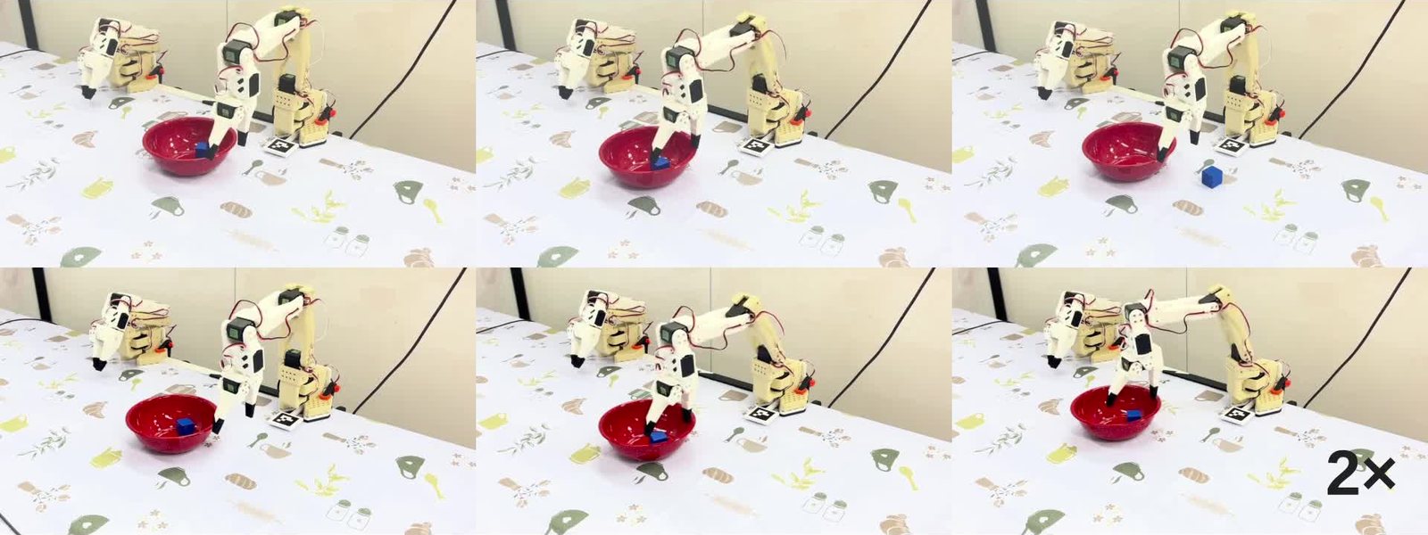
Five of six is a demonstration, not a rate. The 95% Wilson interval on 5 of 6 runs from 44% to 97% (Reasoned). The paper's own limitations section says as much: one task, six trials.
The cost is the other number in that section. Running MCTS in the twin took 644.72 seconds per trial on average, close to eleven minutes before the arm moves (Reported). The authors also distilled the search: 120 successful trajectories from MCTS in randomized sim scenes trained an ACT policy by behaviour cloning, which also scored 5 of 6 and cut the average to 72.306 seconds, about 8.9x faster (Reasoned from the two reported times). Note what the distilled pipeline still does: it rolls the ACT policy out several times in the twin, picks a rollout that succeeds, and replays that open-loop on the robot. The simulator remains the gatekeeper.
What holds, and where it stops
What holds, on the paper's own evidence:
- Spending inference on search raises the rate of finding a passing trajectory, monotonically in budget, with no weight update.
- At equal budget, tree search with step-scored feedback beats independent sampling on average, 65% to 51%, and beats chained refinement, 37%.
- Scores attached to waypoints are the ingredient that makes refinement work; raw rollout images and trajectory text do not.
- Relevant retrieval beats more context.
Where it stops:
- It needs a simulator with a success check, per scene. Every number in the table depends on a ground-truth verifier, and the real-robot result depends on building a twin good enough that sim success predicts real success. The one real failure is a twin-fidelity failure.
- Execution is open-loop. The paper lists this first among its limitations. Nothing corrects a slip once the arm is moving. The FLUX 3 Action piece shows the other end of that trade: a policy that emits a short chunk of actions, then looks again.
- The scorer is the same model as the generator. Gemini Robotics-ER 1.5 proposes, and the same model grades. The final check is the simulator's, so this cannot inflate the table, but it does mean the search is steered by a judge whose errors are correlated with the proposer's.
- Small, single-run evaluation. 20 seeds per task, one run per setting, one real task, six trials.
- No code. The prompts, the discretization, and are not published, so none of this can be re-run.
The pattern is familiar from elsewhere on this site. Adapt-1 Machina also replaced the critic with a simulator and a rewrite of a recorded parent, and paid for it in executed attempts. AIRA found that operator quality, not search sophistication, drove its agents' results, and Interference Search is a reminder to check what a search budget actually counts. SAIL's ablations point the same way as AIRA's from the robot side: the gain comes from a better proposal (the right demonstration) and a better critique (scores on steps), and the tree is how you collect on them. For the orchestration side of Sakana's work, see Sakana Fugu.
The idea worth keeping is the unit of search. Treating a whole trajectory as one node, and a rewrite as one edge, is what lets a model that only knows how to write text do test-time compute on a physical task. It works as well as the simulator it runs in.