Neuron lens: what a neuron's weights say, and what steering it does, checked on a 0.6B model
mdjsonmcp2026-10-31 · 22 min · interpretability · qwen · transformers · small-models

Why read this
Hightop 30%Explains the J, R, K and S lenses from the methods notes and re-runs the steering and input-side checks on Qwen3-0.6B with held-out documents and controls.
- Interactive explanations
- Original analysis
- Runs on a laptop CPU
InterpretabilityCC-BY-4.0Research dataset
How this was scored
- Is it new?
- 2 of 3: A real new idea, method or capability
- Can I trust it?
- 2 of 3: Measures key facts from files, code or configs
- Can I run it?
- 2 of 3: Open code or weights with real limits
- Will I understand it?
- 3 of 3: Mechanism carried by interactives built from real code or data
- Can I act on it?
- 2 of 3: A concrete recipe, numbers or comparison
- Will it last?
- 1 of 3: Relevant for months
- Does it affect many?
- 1 of 3: A specialist community
- Only here?
- 2 of 3: A teardown or measurement few others did
Score 68 of 100, ranked 173 of 666 rated articles. Each question is answered 0–3 by hand, and a 3 is rare. How articles are scored
On 30 October 2026 two researchers, a9lim and treetown, published Neuron Lens: a public catalog of what every MLP neuron and every attention head in two open models responds to, and what it makes the model say. Qwen3-8B has 36 layers of 12,288 neurons and 32 heads, which is 442,368 neurons and 1,152 heads. Gemma 4 12B has 48 layers of 15,360 neurons and 16 heads, which is 737,280 neurons and 768 heads. Each unit is read three ways: from its weights through two Jacobian lenses, from its activations over 15 million tokens of web, Chinese, Python and chat text, and from the exact tokens that drive it. Claude Haiku 5.5 then wrote a label for every pole, at a reported cost of $105 for the 884,736 poles of Qwen3-8B (reported; the sums are mine). The data is CC BY 4.0, the site is AGPL-3.0.
I wrote about finding a neuron and steering it a few days ago, on a small model. That article asks what happens when you push a neuron. This catalog asks the earlier question: what does the neuron say it is for, and can you tell from the weights alone? The authors report that you often can. I wanted to see how much of that survives on a model I can run on a laptop CPU, so this page explains the lenses from the authors' methods notes, summarises what they claim and how they checked, and re-runs two of their checks on Qwen3-0.6B with my own code, on held-out documents with controls.
- license
- MIT
- branch
- main
- tests
- 4 files
- source
- 738.3 kB
- commit date
- 2026-10-30
by size of tracked source at this commit, file counts in brackets; docs, data and vendored trees excluded
local clone, 2026-10-31 at 07fdf45 — branch, commit, commitDate, fileCount, hasTests, languages, license, licenseFile, shallow, testFileCount
shallow clone: counts describe the pinned tree, not the history
- architecture
- Qwen3ForCausalLM
- task
- text-generation
- library
- transformers
- license
- apache-2.0
- safetensors
- 1 shard
- largest file
- 1.50 GB
- files
- 10
- downloads
- 23.7M
- likes
- 1.9K
repo last modified 2025-07-26
A neuron has two poles, a read and a write
A transformer block's MLP in Qwen3 is a SwiGLU. Neuron of layer is coordinate of the input to down_proj. It looks at the normalised MLP input through two rows, one from the gate projection and one from the up projection, with the norm's weight folded in:
and it adds back into the residual stream. That last vector is the neuron's write. The pair of rows is its read.
Because the up projection is linear, act takes both signs. The gate has to be open, so has to be positive, and then the sign of the activation is the sign of . The authors treat the two signs as two poles of one neuron and catalogue them separately. The positive pole reads along and writes . The negative pole reads along and writes (hats are unit vectors). The notes call the read direction a heuristic: the gate and up rows are nearly perpendicular, with a median cosine of 0.00 at every layer of Qwen3-8B except the third, so the two poles really do read different directions. The activations decide which pole fires in practice (reported).
This is also why my steering article adds a signed multiple of one column of down_proj: the write of a pole is a fixed direction, and steering a pole just supplies the activation by hand.
Three ways to read a vector inside a model
A lens turns a vector inside the model into a ranking over tokens. The oldest is the logit lens: pretend the vector is already at the output and read it as , where is the final RMSNorm and the unembedding. It works near the top and reads noise early, because the layers above transform the vector heavily.
The J-lens of Gurnee et al. keeps those layers by linearising them. Let be the residual at position after layer , and the last layer's output before the final norm. The matrix
is the Jacobian of the final residual with respect to layer 's, summed over the current and later positions (so effects carried by attention count) and averaged over a corpus. The read is : what makes the model say, on average, once everything above has acted on it.
The K-lens, from Theia Vogel, takes the Jacobian the other way, back to the input embeddings :
which answers a different question: which input tokens, at this position or earlier, put this direction there. The R-lens and S-lens are the J-lens and K-lens computed under RelP's propagation rules instead of the true gradient: the norm scales are held constant, is linearised as , and the product of gate and up passes half of each factor's change. The authors fit both on 1,000 documents of 128 tokens, at about 11 seconds a document per lens for Qwen3-8B on one H100 (reported). One pass per basis direction of the fixed end covers every layer at the other, so either lens costs passes per document.
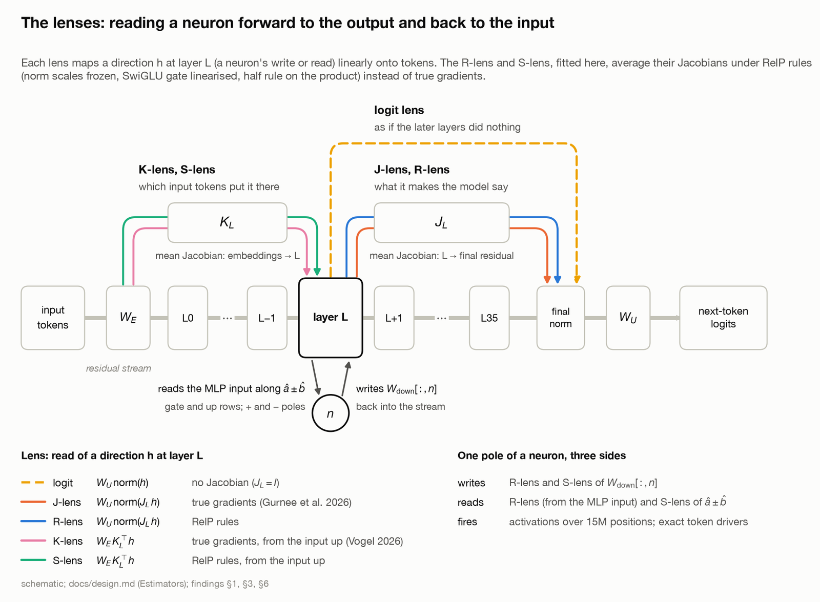
One more rule matters for what a read means. Each lens is fitted at two points of every layer, and the notes state a lens rule: the layer's output (out) reads MLP writes and attention inputs, and the MLP input (mid) reads MLP read directions and attention writes. A read anywhere else extrapolates, and the catalog ships none. Pick a lens and a tap below to see which columns it feeds.
A first-order preview of steering
There is a consequence of the definitions that I worked out while setting up the check below. I have not seen the authors state it, so I label it reasoned. Add a vector at layer at every seed position at once and measure the change in the final residual. To first order the change at position is , because attention is causal. Sum that over and divide by the number of seeds and you get for that document. So the J-lens read of a neuron's write is a corpus-averaged, first-order preview of steering the neuron at every position, read through the unembedding. It also needs no fitted matrix: a central finite difference of the final residual gives it in two forward passes. That is how I compute it below.
It also says where a lens must fail. Steering adds a push of a particular size, and the response of the model to a large push is not linear. A weight-only read is a statement about the direction of the push for small pushes.
What the catalog contains
Every neuron has a and a pole, so Qwen3-8B has 884,736 neuron entries and 1,152 heads, and Gemma 4 12B 1,474,560 neuron entries and 768 heads. Each gets five tables: reads (the weight-only lens reads, each keeping its top 64 tokens), acts (how hard and how often it fires, and its top contexts), drivers (the tokens that make it fire, found by substituting every common token at one position of 8 real documents), legible (which reads hold at the unit's own top firings) and labels (Haiku's labels in words with a confidence). Gemma 4 12B, which also takes images and sound, adds image and audio tables, with its neurons read through 49,694 labelled images and 46,932 labelled sounds, and a media table for heads (reported).
The explorer addresses every view as a path, for example /qwen3-8b/L8/n344 for neuron 344 of layer 8, and draws it in the browser. It serves no unit's data as text, so to look something up you read the Parquet tables in the dataset on Hugging Face, and the lenses are in stdlogits/rs-lenses. The README shows what a row says. L8 n344 + fires on "the sound of the⟦ ow⟧ls", its exact drivers are owl, Owl, OWL and Athena, the R-lens read of its input is owl, 星空 (starry sky) and Owl, and the R-lens read of its write is owl, noct, bedtime and night. L35 n9510 + fires on hashes and IDs, and the notes say it writes no token at all: it sets the temperature of the output (reported).
Which read to trust where. The authors measured that no single read works at every depth, and the map is the most useful part of the write-up for a reader who wants to use the catalog. For Qwen3-8B (reported):
| layers | what drives a pole | what a pole writes |
|---|---|---|
| L0–L7 | the S-lens read of its read direction: literal tokens | the S-lens read (early neurons write back the tokens they detect); the R-lens from about L4 |
| L8 | both lenses, agreeing most | both |
| L9–L12 | the R-lens read: concepts; and exact drivers | the R-lens read: what steering does, rarely what follows a firing |
| L13–L20 | only exact drivers and activations: 82% of poles pass no weight-only test here | the R-lens read, for steering |
| L21–L35 | the R-lens read, often the word about to come | the next token from about L23, suppression from L32 |
What the authors report, and how they checked it
The findings document gives each result its setup, controls and limits, which is more than most releases do. The ones that matter here, all reported:
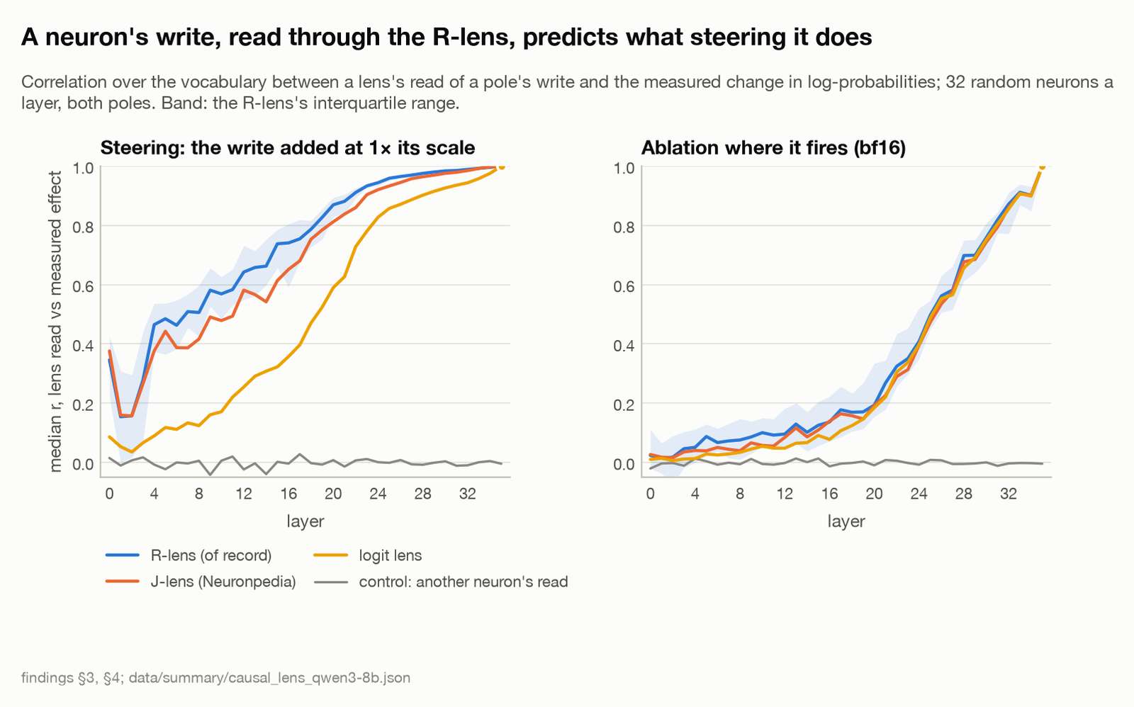
- A write's lens read predicts what steering it does. They add a pole's write to 48 positions of 16 held-out documents and correlate the change in next-token log-probabilities with the lens's read of the same vector. The R-lens reaches a median Pearson r of 0.46 to 0.51 at L4–L8, 0.64 to 0.74 at L12–L16 and 0.9 or more from L22, against ±0.04 for another neuron's read. The plain logit lens trails until about L20 (L8: 0.12 against the R-lens's 0.51).
- Steering is not what a firing does. Before L22, only 1 to 4% of poles promote the tokens that follow their top firings, against 31 to 32% at L28–L29. A firing's effect depends on context before L21: the same pole firing equally hard pushes predictions different ways in different documents.
- Most mid-network neurons are dark to weight-only reads. Of the poles, 38% are read by some test, 5% are silent, and 57% are dark: they fire, but no token-level test passes (82% of L13–L20).
- The labels are checked blind, and the checks are modest. For 100 Qwen3-8B poles, a firing label picks out held-out top firings at AUROC 0.82 (another unit's label: 0.56), and a judge picks the write label out of four 61% of the time (chance 25%). The Gemma 4 12B neuron labels are not checked yet, and its head write labels are picked 22% of the time against a chance of 25%, which the site says to read as guesses.
- Outside labels. The authors also judged an independent persona library, which labels poles by steering each one while the model answers "Who are you?". On 360 rows judged blind, 34% of its personas clearly match the pole's write read, against 2 to 5% for swapped names, and labels from one steering prompt are the ones activations most often contradict. A single prompt can mislead.
Re-running two checks on Qwen3-0.6B
I wrote scripts/neuron-lens/lens_check.py (it is in the repo with the other files for this article) to re-run the idea of two checks on Qwen3-0.6B, which has 28 layers, a 1,024-dimensional residual stream and 3,072 neurons a layer. I sampled 4 random neurons at each of 9 depths (L0, 2, 4, 8, 12, 16, 20, 24 and 27), which is 36 neurons and 72 poles. All documents are windows of this site's own article text, in three disjoint sets: 100 documents of 96 tokens (9,600 tokens) for activations and top firings; 4 documents of 64 tokens, where the lens reads are taken; and 8 other documents of 64 tokens, held out, where steering is measured. As in the authors' setup, seeds sit at positions 16 to 62, so the first 16 positions (the attention sink) are left out. The candidate vocabulary is the tokens seen at least three times across the text of every article on this site, 29,636 of them (the authors keep 103,830 of 151,669).
The differences from the authors' pipeline are large, and every one of them makes my numbers noisier or less comparable:
- I use the true derivative, so my reads are J-style and K-style, not R-lens and S-lens.
- I fit no matrix. A J-style read of a vector is a central finite difference: add at the seed positions of the four lens documents, with set to 2% of the residual norm, and take the change of the final residual, averaged over seeds and documents (two forward passes, the derivation above). A K-style read is one forward and one backward pass.
- Four documents of 64 tokens, where they fit on 1,000 of 128.
- My lens documents and held-out documents come from the same small pool of technical English.
The weights stay in bf16, which is how the checkpoint is stored, and each matrix is upcast to fp32 inside its own matmul, because the shared machine had little memory to spare. That reproduces the fp32 model exactly. As a check, its logits correlate 0.9999 with the plain bf16 model's on a test prompt and the top token agrees at every position (measured).
The script runs in four stages, acts, reads, dose and summarize, each resumable:
QWEN_DIR=<Qwen3-0.6B snapshot> NLENS_OUT=<dir> nice -n 19 python scripts/neuron-lens/lens_check.py actsThe per-neuron records, the dose runs, the summary and the list of documents used (file names and token counts only) are in results.json, reads.jsonl, dose.jsonl and docs-provenance.json.
Check 1: does a weight-only read of a write predict what steering does?
For each pole I add its write, times the pole's typical top activation (the median of its 30 strongest firings over the 9,600 tokens), at the output of layer at the seed positions of the 8 held-out documents. I record the mean change in log-probability of each of the 29,636 tokens and take the Pearson correlation with each lens's read of the same write. The control correlates a neuron's steering effect with another sampled neuron's read from the same layer. The authors run the same test, on Qwen3-8B, with 16 documents and doses of 1× and 4× a pilot estimate of the typical activation (reported).
| layer | push at 1× (× residual) | logit lens r | J-style r | control r | J-style r at 4× | J-style r at 16× (push × residual) |
|---|---|---|---|---|---|---|
| L0 | 0.04 | 0.10 | 0.53 | 0.03 | 0.52 | 0.33 (0.71) |
| L2 | 0.03 | 0.10 | 0.57 | 0.01 | 0.57 | 0.46 (0.52) |
| L4 | 0.02 | 0.17 | 0.67 | −0.06 | 0.66 | 0.61 (0.35) |
| L8 | 0.02 | 0.28 | 0.80 | 0.10 | 0.80 | 0.72 (0.35) |
| L12 | 0.02 | 0.31 | 0.84 | 0.00 | 0.83 | 0.77 (0.25) |
| L16 | 0.02 | 0.55 | 0.91 | −0.03 | 0.90 | 0.84 (0.31) |
| L20 | 0.02 | 0.69 | 0.97 | −0.02 | 0.97 | 0.95 (0.38) |
| L24 | 0.02 | 0.88 | 0.99 | −0.01 | 0.99 | 0.98 (0.35) |
| L27 | 0.03 | 1.00 | 1.00 | −0.01 | 1.00 | 1.00 (0.45) |
Table: median over 8 poles a layer, measured on Qwen3-0.6B. At L27 the last layer's output is the final residual, so the J-style read is the logit lens and r is 1.00 for both. That row checks my code and is not a result.
The shape is the authors' shape. The J-style read predicts steering from the first layer, with median r of 0.53 at L0, 0.67 at L4, 0.80 at L8, 0.91 at L16 and 0.99 at L24. The plain logit lens starts at 0.10, is still at 0.28 at L8 and 0.55 at L16, and only catches up in the last quarter of the network (0.88 at L24). Another neuron's read stays between −0.06 and 0.10. On Qwen3-8B the authors report 0.09, 0.12 and 0.36 for the logit lens at L0, L8 and L16, and 0.38, 0.42 and 0.65 for the J-lens (reported), so the ordering and the gap agree. My values are higher early on, probably because my lens and test documents are the same kind of text and my pushes at 1× are only 0.02 to 0.04 of the residual stream, which keeps the response close to linear. I did not test either explanation.
The dose columns show where the first-order read stops working. At 4× the J-style correlation is the same to two digits at every layer. At 16×, a push of 0.25 to 0.71 of the residual stream, it falls at the early layers: 0.33 at L0, 0.46 at L2, 0.61 at L4, 0.72 at L8 and 0.77 at L12, and it stays at 0.84 or above from L16. That is what a linearisation should do: a read of the direction is a statement about small pushes, and the early layers have the smallest residual norms and the most layers above them to bend the response. At the same small dose the read is still weaker at L0 than at L8, and a bigger dose makes it worse.
Noise is the other limit, and it is large here. Splitting my four lens documents into two halves of two, the two J-style reads of the same write share on average 3% of their top-10 tokens at L0, 25% at L4, 18% at L12 and 42% at L20, and reach 82% at L24 and 100% at L27. The authors report that the R-lens read of a write has the same top token across halves of 500 documents for 89 to 99% of neurons (reported). Pearson r over 29,636 tokens survives a noisy read because it is dominated by the broad shape of the change, and the authors say so too. The top-10 lists are another matter: the logit lens and the J-style read share 0% of their top 10 at L0 and 5% at L16, and only 40% at L24.
Check 2: does an input-side read find the tokens that fire a pole?
A pole reads along . For each pole I take the tokens at its 20 strongest firings over the 9,600-token activation corpus (those in the candidate vocabulary), and count how many land in the top 10 or top 50 of four reads of that direction: the K-style read (one backward pass from the layer to the embeddings), the plain projection on the token embeddings, the J-style read of the direction, and a control, another neuron's K-style read from the same layer.
| layer | K-style top 10 | K-style top 50 | embedding top 50 | J-style top 50 | control top 50 |
|---|---|---|---|---|---|
| L0 | 2% | 11% | 6% | 0% | 6% |
| L2 | 2% | 9% | 5% | 0% | 0% |
| L4 | 5% | 7% | 3% | 0% | 0% |
| L8 | 0% | 0% | 0% | 6% | 0% |
| L12 | 0% | 0% | 3% | 1% | 0% |
| L16 | 1% | 1% | 1% | 3% | 0% |
| L20 | 0% | 3% | 2% | 4% | 0% |
| L24 | 0% | 0% | 0% | 0% | 0% |
| L27 | 1% | 1% | 1% | 1% | 0% |
Table: share of a pole's firing tokens found in the read's top 10 or top 50, mean over 8 poles a layer, measured.
These are small numbers from small samples. A layer is 8 poles and about 20 firings each, so one pole moves a layer's rate by several points, and I would not call this a replication. What it shows is the sign. The K-style read is above both the embedding shortcut and the control at L2 and L4 (9% and 7% in the top 50, against 5% and 3%, and 0% and 0%), at L0 it gets 11% against 6% for the shortcut and for the control, and from L8 on it finds at most 3%, against 0% for the control. That fits the authors' report that the S-lens read works at the lowest layers and fades after L8 (reported). My absolute rates are far below theirs, who find 40% of firing tokens in the top 10 at L0 and 2 to 9% at L1 to L8. I would blame the 29,636-token vocabulary, the four lens documents and the narrow text, in that order of confidence, but I did not separate them.
What the reads look like
The table below is built from the same files. It shows, for the + pole of one sampled neuron per depth, the tokens it fires on and what each read says. The neuron at each depth is the one whose input reads found the most of its firing tokens, so these are the best cases, not typical ones. Most neurons look like the one at L2 or L8.
At L4 the pole fires on spend and time. The K-style read of its input is investment, budget, spending, spend. The J-style read of its write includes investment, Spending, spent and money, and measured steering raises investment, pricing, budget, market, while the plain logit lens of the same write gives rices, carefully and protect. At L12 the J-style read of the write ( consumers, testers) is the measured steering effect, and the logit lens gives word fragments. At L27 the pole fires on − and delta, and the K-style read of its input is Delta, Δ and offset. The L8 neuron is the honest counter-example: the J-style read of its write and the measured steering share cybersecurity and little else.
What I take from it
A weight-only read of a write is a usable preview of steering in the second half of the network, a noisy one in the first, and the plain logit lens is a poor stand-in until the last quarter, which agrees with the authors. The finite-difference read I used is not cheaper than steering: it costs two forward passes a candidate, where measuring the steering effect costs one. What makes the authors' version cheap is the fitted lens. Once is fitted, reading a write is a matrix-vector product, so all 86,016 neurons of a model this size cost almost nothing, and steering has to be run only for a shortlist. I did not test that shortlist, and the authors' own point stands that a good steering preview says nothing about what a neuron does when it fires, because the effect of a real firing depends on context before about L21.
What I did not run
I did not run the authors' pipeline, their explorer or their code, and I did not load Qwen3-8B or Gemma 4 12B, so none of the catalog's own numbers is re-checked here. I used true gradients where they use RelP's rules, so nothing below says anything about the R-lens or S-lens themselves. I did not fit a lens matrix, I did not re-label anything, and I did not test the ablation check or the head circuits. The documents come from this site's own articles, which are narrow, technical English with some code.
Sources
- Neuron Lens, neuron-lens.com, the research README, findings and methods; the catalog on Hugging Face and the lenses on Hugging Face; the announcement thread by a9lim and treetown.
- Lenses the notes build on: the logit lens (nostalgebraist, 2020), the J-lens (Gurnee et al., 2026), the R-lens (camilablank et al., 2026), the K-lens (Theia Vogel, 2026) and RelP (arXiv:2508.21258).
- My earlier article on finding a neuron and steering it.