Model casting: compute the gate, then skip most of the FFN

2026-10-02 · 17 min · explainer · llm · inference-optimization · transformers · efficiency · mixture-of-experts

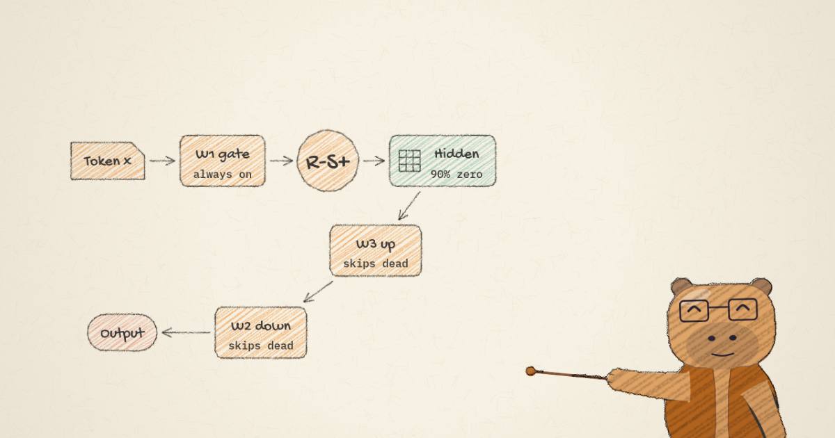
The feed-forward network is the part of a transformer that nobody talks about and everybody pays for. Attention gets the papers; the FFN gets the FLOPs. In a modern SwiGLU block the FFN holds roughly two-thirds of the non-embedding parameters, and every one of them runs on every token. The uncomfortable part is that most of that work is already wasted: for any given token, the large majority of the FFN's hidden units contribute almost nothing. The activations are nearly sparse. We just can't cash it in, because the activation function the whole industry switched to — SiLU — produces small numbers, not exact zeros, and you can't skip a matmul whose inputs are merely small.

Model Casting and Low-Parameter Gating (Lomeli et al., Meta FAIR and ENS, September 2026) is about making that sparsity real and then spending it. It is a mid-training recipe: take a pre-trained model, swap the FFN activation for one that zeroes the negative half, add a penalty that drives the sparsity to an explicit target, and keep training. At inference you then compute the gate first and, because ~90% of its outputs are zero, skip the two other FFN matrices for the dead units. That is up to a 3x cut in FFN FLOPs. A second idea, LoPA Gating, makes the gate itself cheap and pushes past the 3x ceiling that every activation-sparsity method hits. On a 5.8B model with custom kernels the authors report a 3.31x wall-clock speedup on the FFN at 90% sparsity.

No code or weights have been released, so everything here is a read of the paper and its figures, not a reproduction. Where I give a number I say whether it is reported (the authors' measurement), reasoned (my arithmetic on their formulas), or measured (something I computed from an artifact myself). There are no measured numbers in this one — there is nothing to run.

What an FFN actually computes

Strip a transformer block down and the FFN is two or three matrices with a nonlinearity in the middle. Modern models use the gated form (SwiGLU and its cousins). On a single token's hidden vector $x \in \mathbb{R}^{D}$ , a gated FFN of hidden width $H > D$ computes

y = W_2\,\bigl(A(W_1 x) \odot (W_3 x)\bigr),\quad W_1, W_3 \in \mathbb{R}^{H \times D},\ W_2 \in \mathbb{R}^{D \times H}.

Three matrices. $W_1$ is the gate: its output goes through the activation $A$ . $W_3$ is the up projection. The two are multiplied element-wise ( $\odot$ ), and $W_2$ projects the result back down to width $D$ . Each matrix costs $HD$ multiply-adds per token, so a dense FFN costs $3HD$ . With the usual ratio $H = 8D/3$ , that is $8D^2$ parameters in the FFN against roughly $4D^2$ in attention — which is where the "about two-thirds" comes from (reasoned). Grouped- query attention, which this paper's base architecture uses, makes the FFN's share larger still.

Here is the lever. The vector $A(W_1 x) \in \mathbb{R}^{H}$ has one entry per hidden unit. If entry $i$ is zero, then hidden unit $i$ is dead for this token: its contribution to the element-wise product is zero, so you never needed row $i$ of $W_3$ , and its zero contribution to the sum means you never needed column $i$ of $W_2$ either. Skip both. The only catch is timing, and it is the whole story of this paper.

Sparsity you can't spend

"Activation sparsity" means exactly this: for a given token, most hidden units output ~0. It is not a design goal anyone added — it falls out of training. When the activation is ReLU, a trained transformer produces genuinely sparse intermediate activations on its own, and the effect grows with training data (Li et al., 2023; Luo et al., 2025, as cited). ReLU hands you exact zeros for free: everything below the threshold is identically zero, and a zero is a thing you can test for and skip.

The problem is that nobody trains with ReLU anymore. The field moved to gated SiLU and GELU FFNs because they are better, and they are — but $\text{SiLU}(x) = x\,\sigma(x)$ is smooth and never exactly zero for finite $x$ . A SiLU gate produces small numbers, not zeros. You cannot skip a matmul because its input is 0.001. So the sparsity is still there in spirit — most units are near-dead — but there is no clean boundary to exploit, and pre-training from scratch with ReLU instead risks neurons that die permanently and never come back.

This is why the interesting work happens at mid-training: start from a good SiLU checkpoint and recover the exploitable sparsity without paying to pretrain from scratch. Prior mid-training approaches swap the activation to ReLU when fine-tuning (RELU-fication, Mirzadeh et al., 2024). The trouble is that the attainable sparsity is then whatever the swap happens to give you — it is a side effect, not a target you set. Training-free methods that threshold the SiLU gate at inference (TEAL, top- $p$ ) are bounded by the sparsity the frozen model already admits; one such method reports a critical sparsity — the level reachable at a 1% quality drop — of at most 40% for an 8B model (reported). Model casting's pitch is that you should be able to ask for 90% and get it.

The 3x ceiling, and why W1 is always on

Before the recipe, the arithmetic that bounds it. A zero is exploitable only if you know it is zero before the matmul it feeds. The gate's zeros live in $A(W_1 x)$ , which you only have after computing $W_1 x$ in full. So $W_1$ always runs. What the zeros buy you is $W_3$ (you skip the dead rows) and $W_2$ (you skip the dead columns). Writing $s \in [0,1]$ for the sparsity fraction and $\text{cost}(W)$ for the multiply-adds actually executed:

\text{FLOP-ratio} = \frac{3HD}{\text{cost}(W_1) + \text{cost}(W_2) + \text{cost}(W_3)} = \frac{3HD}{HD + 2(1-s)HD} = \frac{3}{3 - 2s}.

At $s = 0.9$ that is $3/1.2 = 2.5\times$ ; at $s = 0.95$ it is $2.73\times$ ; and as $s \to 1$ it approaches $3\times$ and no further (reasoned, from the paper's Eq. 2). That $3\times$ is a hard ceiling for any method that keeps a full gate matrix, because one of the three matrices can never be skipped. The paper's name for this is the always-on cost of $W_1$ .

The widget below is that formula, made adjustable. Drag the sparsity up and watch the two skippable matrices shrink while the gate holds firm; the speedup climbs toward 3x and stalls. Then flip to the LoPA gate (the next section) and watch the ceiling move.

Compute the gate first, then skip the dead units

Activation sparsity90%

Hidden units after A(W1·x)4/40 active

W1 gate

low-rank (r = D/8)

7.4%

W3 up

skips dead units

4.6%

W2 down

skips dead units

4.6%

FFN FLOPs

17%

of a dense FFN

FFN speedup

6.02×

breaks 3× — up to 13.5×

NLL cost

+0.93%

measured @ 89% (Table 1)

FLOP shares are exact arithmetic from the paper’s formulas (dense = 100%; H = 8D/3, rank ratio α = r/D = 1/8). The speedup is the reciprocal of the FFN’s remaining FLOPs. The NLL cost is not modelled: it snaps to the nearest measured 0.81B operating point and is blank where no cast model was measured. Saved 83% of FFN FLOPs at this setting.

Model casting: make sparsity a target

The recipe has two independent ingredients, and you can use either alone.

First, the activation. Replace SiLU with R-S+, a hybrid that equals SiLU on the positive side and zeroes the negative side:

\text{R-S+}(x) = \begin{cases} x\,\sigma(x) & x \ge 0 \\ 0 & x < 0 \end{cases}

The design is deliberately conservative. Because R-S+ coincides with SiLU for $x \ge 0$ , casting only perturbs the negative half of the activation — the part that was already contributing least. RELU-fication, by contrast, changes the function across the whole input range and forces a larger adaptation, which is why it costs more quality for less sparsity. You start from a checkpoint while the learning rate is still stable, swap every FFN's activation to R-S+, reset the optimizer state, and resume with a short warm-up before decaying.

Second, the penalty. The activation swap alone does not get you to 90% — applied mid-training it lands well short. So model casting adds an $\ell_1$ penalty on the hidden activations and makes it adaptive. The loss is

\mathcal{L} = \mathcal{L}_{\text{CE}} + \frac{\lambda}{H}\sum_{\ell=1}^{L} \bigl|\mathbf{h}^{(\ell)}\bigr|_1,

where $\mathbf{h}^{(\ell)} = A(W_1 x)$ is the FFN activation at layer $\ell$ . Bigger $\lambda$ means sparser activations but higher cross-entropy — a direct quality-for-sparsity dial. Rather than guess $\lambda$ , they target a sparsity $s^{\star}$ and let $\lambda$ chase it: $\lambda_{i+1} = \lambda_i \cdot \alpha^{\,\text{sign}(s^{\star} - s_i)}$ , nudging $\lambda$ up when the measured sparsity is below target and down when it overshoots ( $\lambda_0 = 10^{-3}$ , $\alpha = 1.03$ ). That is the sense in which sparsity becomes an explicit training target instead of an emergent accident. Set $s^{\star} = 90\%$ and the model arrives at about 89% measured.

Three side-by-side FFN schematics showing FLOPs per matrix. Left, Dense SwiGLU: three trapezoids each labelled 18.3 M, with a full row of beige hidden units and multiply nodes. Middle, Sparse SwiGLU: the gate matrix still 18.3 M, but the up and down matrices drop to 1.8 M each, and most hidden units are now red zeroed squares. Right, Sparse LoPA Gating: the gate is drawn as a low-rank bottleneck at 4.9 M while the up and down matrices are 2.5 M each, over a wider row of hidden units, again mostly red and dead. — Where the FLOPs go. Dense (left): three matrices at 18.3 M each. Sparse standard gating (middle): the up and down matrices collapse under 90% sparsity, but the gate W1 stays at full cost — the 3x wall. LoPA (right): the gate is made low-rank and cheap, and the saved parameters are spent on a wider hidden layer, so the skippable matrices carry more of the budget (Model Casting, Figure 2).

LoPA Gating: moving the ceiling

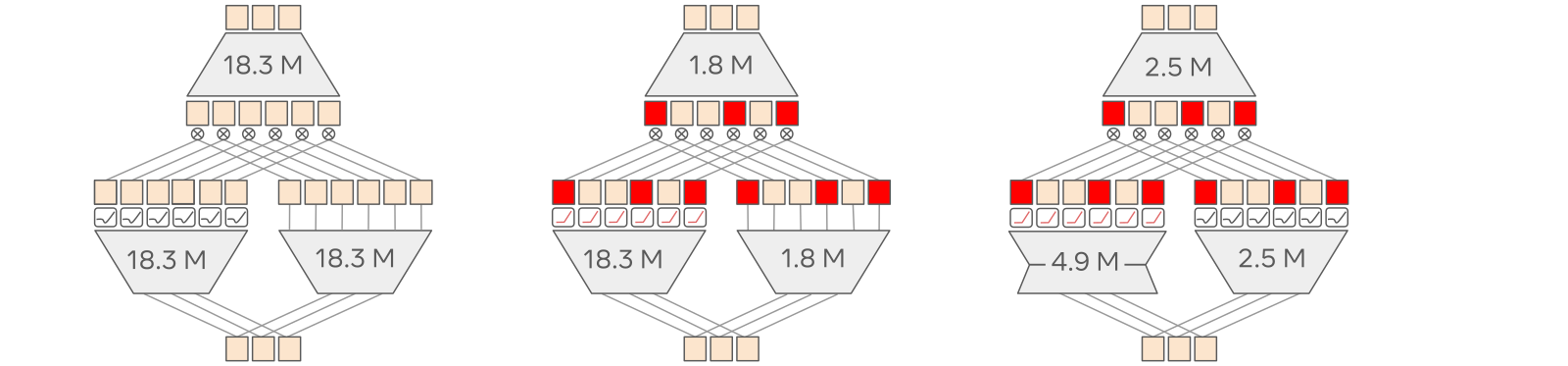
The $3\times$ ceiling exists only because $W_1$ is a full $H \times D$ matrix that always runs. So make it smaller. LoPA Gating (Low-Parameter Gating) reparameterizes the gate as a low-rank term plus a fixed sparse one:

W_1 = G + UV,\quad U \in \mathbb{R}^{H \times r},\ V \in \mathbb{R}^{r \times D},

with rank $r = \alpha D$ (default $\alpha = 1/8$ ), and $G$ a non-trainable matrix with a single 1 in each row. The low-rank product $UV$ is what makes the gate cheap: it costs $r(D + H')$ instead of $HD$ . The fixed $G$ is the clever bit — without it, a pure low-rank $W_1 = UV$ is rank-deficient and the FFN loses expressivity; adding $G$ makes $W_1$ full rank again (it generalizes the diagonal-plus-low-rank trick of Chen et al., 2026 that restores the universal approximation property) at no extra FLOPs or parameters.

Two practical fixes make it trainable. Factoring $W_1$ into two matrices deepens the network and destabilizes large-scale training, so they insert an RMSNorm between the low-rank terms: $W_1(x) = Gx + U\cdot\text{RMSNorm}(Vx)$ . And because shrinking the gate before the activation weakens the FFN's only nonlinearity, they apply the activation to the outputs of both $W_1$ and $W_3$ (double activation), which recovers — slightly exceeds — standard gating.

The payoff is that the parameters you save on the gate get redistributed: the hidden width grows from $H$ to $H' = D(3H - r)/(r + 2D)$ to hold the total parameter count fixed. Now the two skippable matrices carry a larger share of the budget, and the always-on gate carries a tiny one. Plugging the LoPA costs into the FLOP-ratio (the paper's Eq. 4) and using $H = 8D/3$ , $\alpha = 1/8$ :

at $s = 0.9$ , the FFN FLOPs drop by 6.02x (reasoned; matches the paper's Figure 4);
as $s \to 1$ , the ceiling is no longer 3 but about 13.5x (reasoned), because the gate is now ~7% of a dense FFN's cost instead of 33%.

That is the one-line reason LoPA matters: the cap on activation-sparsity speedups was the gate, and LoPA makes the gate almost free.

The paper combines these into three recipes. Activation Casting keeps a full gate and only swaps the activation (ceiling 3x). LoPA Casting pretrains with the LoPA gate from scratch, then casts the activation — same parameter count, faster inference, but you have to own the pretraining. Architecture Casting converts an off-the-shelf model's full gate into a LoPA gate at casting time by fitting $G + UV$ to the existing $W_1$ with alternating minimization, so you can LoPA-ify a checkpoint you did not train (they do this to Qwen3-1.7B).

What it buys, at what cost

Scatter plot of NLL (y-axis, lower is better, 2.145 to 2.166) against theoretical FFN speedup (x-axis, 1 to 6, higher is better). The dense baseline sits at 1x, NLL 2.145. ReLU-fication, top-p and TEAL cluster between 1.4x and 2x with slightly higher NLL. Activation Casting points sit at 1.9x and 2.48x. A dotted green LoPA curve rises from LoPA@50% at 1.9x and low NLL, through LoPA@75% at about 3.2x, to LoPA@90% at 5.83x and NLL 2.165. A vertical dashed line at 3x is labelled max speedup with SwiGLU; the LoPA@90% point sits well to its right. — The frontier. Everything left of the dashed 3x line is bounded by the always-on gate; LoPA@90% sits at 5.83x theoretical FFN speedup for a 0.93% NLL increase over the dense baseline, past a wall the other methods cannot cross (Model Casting, Figure 1).

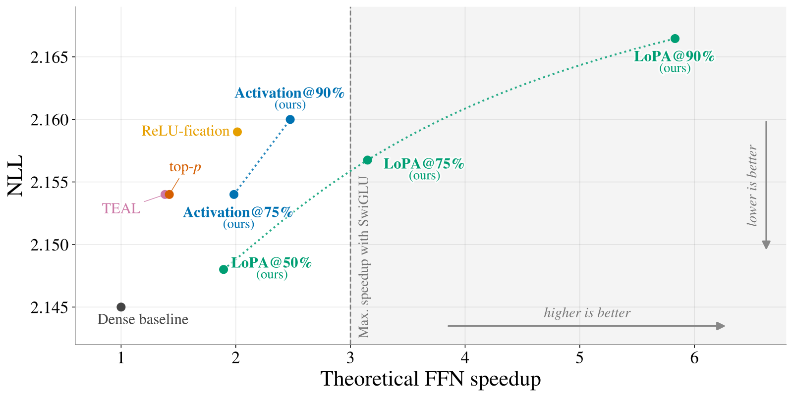
The headline, on a 0.81B model (Table 1, all reported): the dense SiLU baseline scores NLL 2.145. LoPA Casting at an 89% measured sparsity scores 2.165 — a +0.93% NLL increase — for a 5.83x theoretical FFN FLOP speedup. Standard Activation Casting at the same 89% gives +0.68% NLL but only 2.48x, because of the 3x wall. For comparison, at matched quality the best training-free methods (top- $p$ and TEAL) reach only 1.6x, and RELU-fication plateaus below 80% sparsity. Pushing the critical-sparsity frontier from ~40% to ~90% is the real result; the speedup is the consequence.

Theoretical FLOP ratios are one thing; wall-clock is another, and this is where most sparsity papers quietly disappoint. This one does not, with custom kernels: a sparsity-aware AVX-512 kernel on CPU, and Triton kernels on GPU that fuse the $W_2$ and $W_3$ projections and skip the inactive neurons.

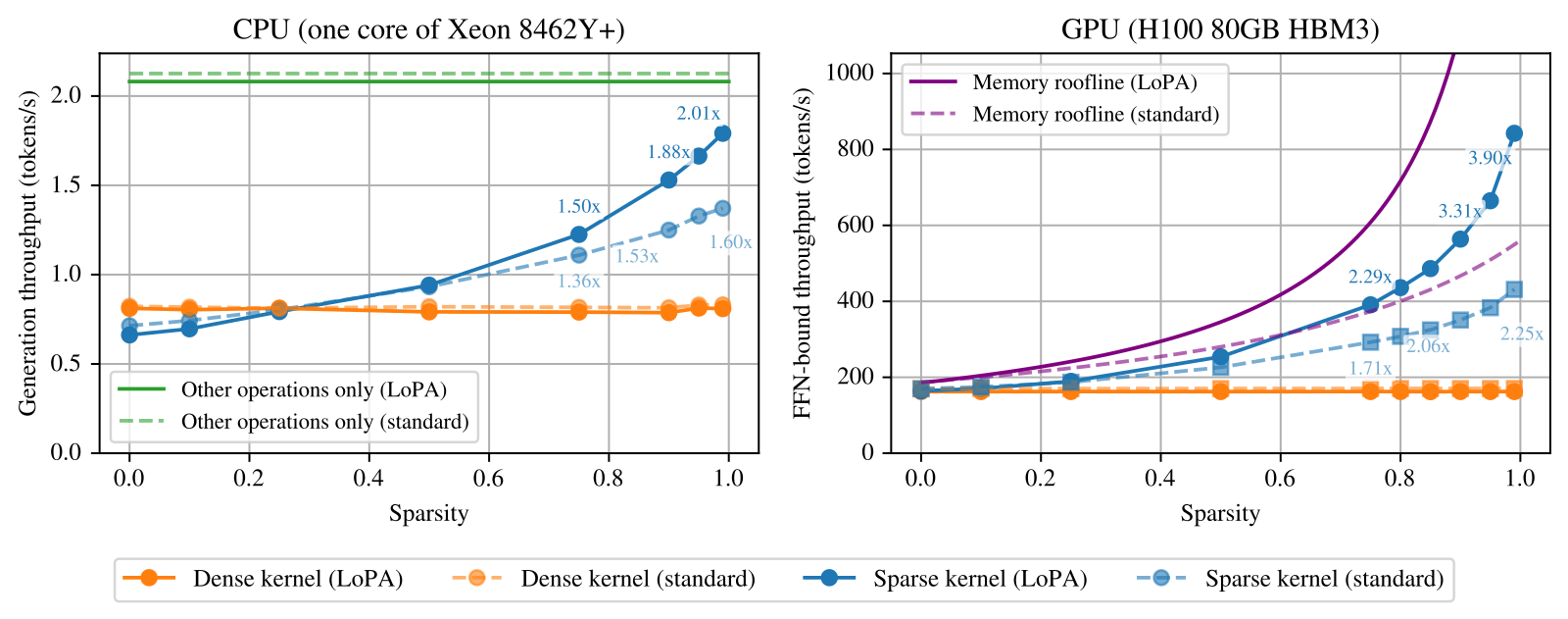
Two throughput-versus-sparsity plots. Left, CPU (one core of Xeon 8462Y+): generation throughput rises with sparsity; at 0.9 sparsity the standard sparse kernel is labelled 1.53x and the LoPA sparse kernel 1.88x, with a dense-kernel flat line near the bottom. Right, GPU (H100 80GB HBM3): FFN-bound throughput rises more steeply; at 0.9 sparsity the standard kernel is labelled 2.06x and LoPA 3.31x, and at 0.95 LoPA reaches 3.90x, below a memory-roofline curve. — Measured throughput against sparsity for a 5.79B model in float32. CPU times are end-to-end on one core of a Xeon 8462Y+; GPU times cover the FFN only on an H100 80GB. At 90% sparsity the GPU FFN speedup is 2.06x for standard gating and 3.31x for LoPA; at 95% LoPA reaches 3.90x (Model Casting, Figure 5).

On the 5.79B model, at 90% sparsity (all reported): CPU end-to-end goes 1.53x (standard) to 1.88x (LoPA); the GPU FFN goes 2.06x (standard) to 3.31x (LoPA), past the 3x ceiling that standard gating physically cannot cross. At 95% sparsity LoPA reaches 3.90x on the GPU while standard Activation Casting is stuck at 3x. The sparsity even stacks with quantization: int8 quantization-aware training on top of a cast model costs 1.57% NLL, and the low-precision sparse kernels reach 8.13x at 90% sparsity against the full-precision dense baseline (reported).

Checking the three claims

The 3x ceiling (reasoned, holds). It falls straight out of the FLOP-ratio $3/(3-2s)$ , which is monotone in $s$ and tends to 3. The only assumption is that $W_1$ cannot be skipped, which is true by construction — you need its output to know where the zeros are. LoPA's escape is equally mechanical: shrink $\text{cost}(W_1)$ and the limit moves. I reproduced the 6.02x at 90% and the ~13.5x limit from the paper's Eq. 4 with $H = 8D/3$ and $\alpha = 1/8$ , and both match the paper's figures.

The 3.31x / 3.90x GPU speedups (reported, plausible). These are the paper's kernel measurements on an H100, FFN-only, and I can't independently time them — no kernels were released. What makes them credible rather than aspirational is that they sit below the memory-bandwidth roofline the authors plot, and that the standard-gating curve lands at 2.06x — just under the 2.5x its FLOP ratio allows at 90% sparsity, where kernel-launch and memory overhead should drag it. The method's internal arithmetic is consistent with its measurements.

The +0.93% NLL at 90% (reported). This is a validation-set number on a 0.81B model, and it is the LoPA Casting operating point. It is worth keeping the asterisk the paper keeps: Architecture Casting — the recipe you would actually apply to a model you did not pretrain — costs more, +2.20% NLL on the same 0.81B model, because converting a full gate to low-rank sheds parameters it cannot grow back. LoPA's clean 0.93% assumes you pretrained with LoPA in the first place. On downstream tasks, Activation Casting costs 0.4 points of a 12-task average at the 90% target, and 1.6 points on Qwen3-1.7B (reported).

Where it generalizes

The gate-is-a-router observation is the bridge to Mixture of Experts. A SiLU gate over hidden units is, structurally, a soft router that decides which units fire — so the same casting mechanism applies to an MoE's expert FFNs and to its router. If you've built an MoE from scratch, the parallel is immediate; see Mixture of Experts, from scratch for the router-and-dispatch machinery this reuses. On an 8-expert top-2 model, casting the expert FFNs reaches 88.6% activation sparsity for +0.083 NLL, and — tellingly — switching to top-1 routing, the usual architectural route to sparsity, lands at a worse NLL with no activation sparsity at all (reported). Casting the FFN and routing the experts are complementary, not competing.

It also composes with the other levers people pull on inference cost. The int8/int4 results put it alongside post-training quantization — the same territory as NVIDIA Model Optimizer, but attacking FLOPs rather than bytes. And where runtime dynamic compression exploits that only a few experts are needed per token to keep memory down, model casting exploits that only a few hidden units are needed per token to keep FLOPs down — two readings of the same conditional-computation idea at different granularities. If you want the ground floor on why the FFN and attention split the work the way they do, how self-attention works covers the other half of the block this one leaves alone.

The takeaway

Activation sparsity was always there; the gated-FFN era spent it without meaning to and then couldn't get it back. Model casting's contribution is to make the sparsity a number you set — ~90%, during a cheap mid-training stage — instead of a number you measure and hope for. The inference trick that cashes it in is old and simple: compute the gate, skip the dead units. The genuinely new piece is LoPA Gating, which notices that the always-on gate was the whole ceiling and makes it almost free, turning a 3x cap into a measured 3.31x and a theoretical 13.5x.

The honest limits are the ones to carry away. The big wall-clock numbers are FFN-only and decode-only; batch the traffic and the win erodes. LoPA's best quality assumes you pretrained with it, and the drop-in Architecture Casting path costs more. And with no code or weights released yet, the 3.31x lives in the paper's plots, not on anyone else's H100. But the arithmetic is clean, the measurements are internally consistent, and the central claim — that you can target 90% activation sparsity and keep the quality — is the kind of result that moves a frontier rather than nudging a benchmark.