2026-10-10 · 30 min · computer-vision · diffusion-transformers · video-understanding · image-generation · benchmarks
Why read this
Notabletop 60%How FreeMatching turns FLUX.2 into a matcher, checked against code and weights: whose baselines its tables use, what the teacher is, and what a pair costs.
- Original analysis
- A lasting reference
- A new technique
Vision & multimodalNeeds a workstation GPUApache-2.0Research paper
How this was scored
- Is it new?
- 2 of 3: A real new idea, method or capability
- Can I trust it?
- 2 of 3: Measures key facts from files, code or configs
- Can I run it?
- 2 of 3: Open code or weights with real limits
- Will I understand it?
- 2 of 3: Mechanism from first principles with figures
- Can I act on it?
- 2 of 3: A concrete recipe, numbers or comparison
- Will it last?
- 2 of 3: A reference for a year or more
- Does it affect many?
- 1 of 3: A specialist community
- Only here?
- 2 of 3: A teardown or measurement few others did
Score 66 of 100, ranked 173 of 494 rated articles. Each question is answered 0–3 by hand, and a 3 is rare. How articles are scored
The post that sent me here was a one-line summary of a new paper: FLUX2-4B plus DINOv3, supervised learning on classical, tracked-video and synthetic datasets, plus teacher-guided iterative refinement. I expected a DIFT-style recipe. Noise an image, run it through a diffusion model, pick a layer and a timestep where the features happen to be good, and match those features with nearest neighbours. Most "diffusion features for correspondence" work since 2023 has gone like that.
FreeMatching does something else. It never adds noise to anything. It takes the whole FLUX.2 transformer, feeds it two clean images as one token sequence, and fine-tunes every weight until the output tokens for the second image decode into a map that says, for each of its pixels, where that pixel came from in the first. There is no layer to pick and the timestep is a constant knob. The diffusion model is used as a very large, very well-initialised two-image transformer.
The paper is Beyond Spatio-Temporal Priors: A Generalizable Approach for Dense Correspondence Matching (arXiv 2610.12421, posted 8 October 2026, accepted at NeurIPS 2026), by Luping Liu, Bingyi Kang, Yifan Wang and Dong Xu, of the University of Hong Kong and ByteDance Seed. The code is at luping-liu/FreeMatching under Apache-2.0, and both checkpoints are on Hugging Face. I read v1 of the paper, every Python file in the repo, and the checkpoint headers.
- license
- Apache-2.0
- branch
- main
- tests
- 1 file
- source
- 368.1 kB
- commit date
- 2026-10-08
by size of tracked source at this commit, file counts in brackets; docs, data and vendored trees excluded
local clone, 2026-10-10 at 20add55 — branch, commit, commitDate, fileCount, hasTests, languages, license, licenseFile, shallow, testFileCount
shallow clone: counts describe the pinned tree, not the history
The short version of what I found: the mechanism is clean and the gains on its own target task are large and show up across several metrics. The "competitive on classical benchmarks" claim is softer than it reads, because the classical tables compare against baselines that were themselves fine-tuned on edited images, and on optical flow FreeMatching trails the flow specialists by a wide margin. And the released code disagrees with the paper on three details that matter if you try to reproduce it.
The task is edits, not video
The title says "dense correspondence", and the summary mentions tracked video, so I went in thinking of optical flow. The paper's real target is narrower and newer. It calls it IEG: image editing and reference-guided generation. You give a model a photo of a horse on grass and ask for the same horse in snow. You give it a photo of a guitar and a seal and ask for a picture of both on a beach. Did the output keep the horse, or a horse? Which pixels of the output are the guitar from the reference, and how well were they preserved?
Answering that needs a correspondence map between the reference and the generated image, and none of the usual tools were built for it.
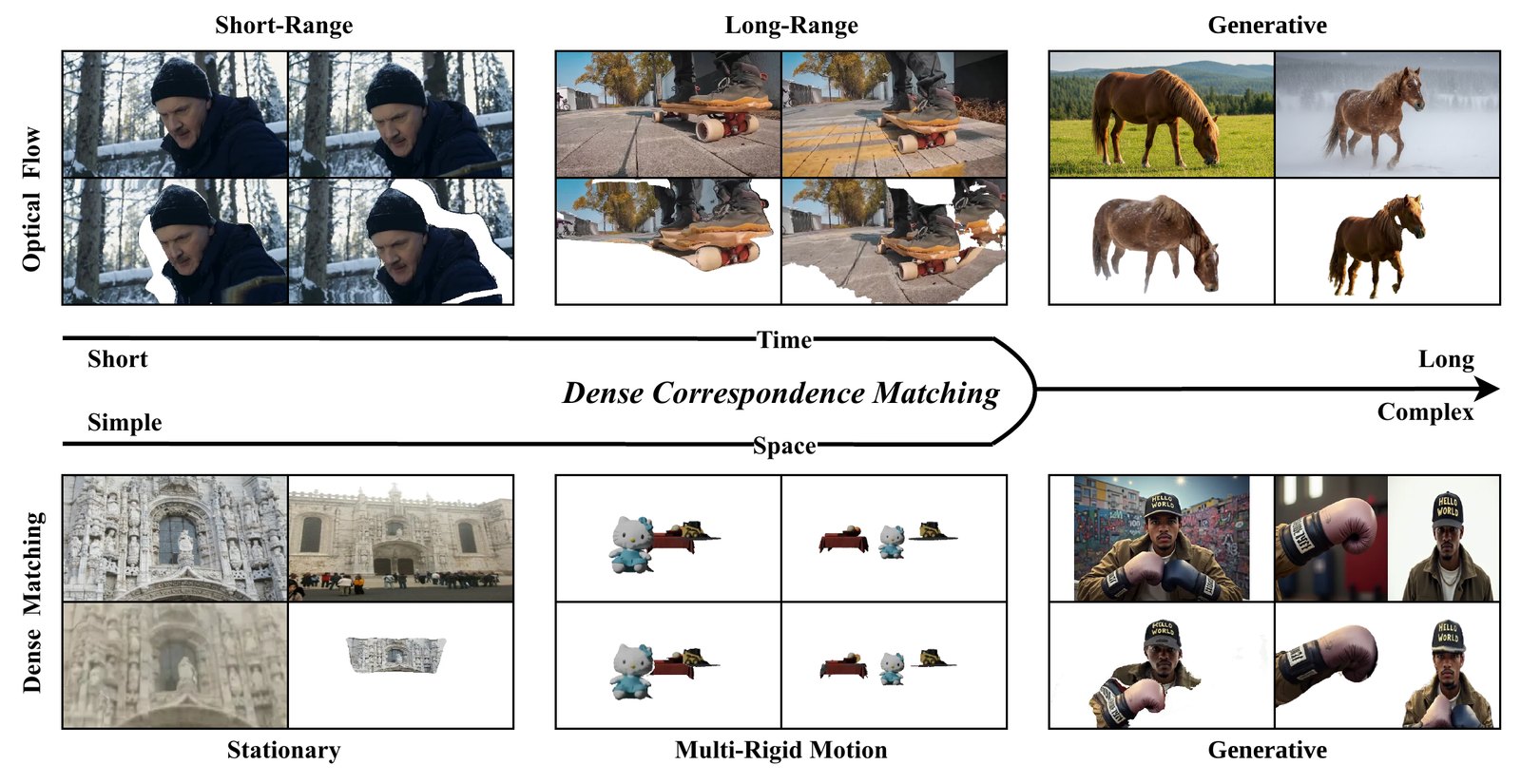
The output is defined precisely. Given a source image and a target , the model predicts a backward map , where says that pixel of the target came from absolute position in the source, plus a covisibility mask in that says whether there is a counterpart at all. Generated content with no source, or background the edit replaced, gets . The direction matters in practice: the released code documents it as "target-to-source", and the warp you get out is the source resampled onto the target's grid.
It helps to put the neighbouring tasks side by side, because the brief I was handed for this article lumped them together and the paper does not.
Optical flow (RAFT, SEA-RAFT, GMFlow) matches consecutive or near-consecutive frames, densely, and is graded in pixels of end-point error. Point tracking (CoTracker, AllTracker) follows points through many frames and has to handle occlusion over time. Wide-baseline matching (RoMa, and the DUSt3R and MASt3R family on the 3D side) matches two views of a static scene where the camera moved a lot. Semantic correspondence (DIFT, SD-DINO) matches different instances of a category: the left ear of one cat to the left ear of another. FreeMatching's target sits between the last two. It wants the same instance, like flow and wide-baseline matching, under the arbitrary transformations of an image model, which is closer to what semantic matchers are used to.
Why the priors break
"Spatio-temporal priors" is the paper's name for two assumptions classical matchers lean on: things do not move far between the two images, and the motion field is smooth, or the scene is rigid. Some of this is architecture. RAFT looks up its correlation volume in a small radius around the current flow estimate and starts that estimate at zero, so it walks toward the answer from the same coordinates. Much of it is data. Every flow dataset is two frames of one physical scene, so a network trained on them learns what physically plausible motion looks like, and treats anything else as noise.
An edited image breaks both at once. The horse can move across the frame. The background around it is new, so nothing near the object's old position matches anything. Its pose changes in a way no camera motion produces.
The explorer below is a toy version of that failure. I built two 32-by-20 "images" out of made-up feature vectors: every cell of an object carries a feature that encodes which object it belongs to and where it sits inside that object, so a point keeps its feature wherever the edit moves it. Background cells carry a feature for "grass" in A and "snow" in B. Click a cell in A and the heatmap over B is the cosine similarity to every cell. Then three readouts turn that heatmap into a single match.
- true match
- (22.0, 8.9)
- local argmax
- (4.0, 0.0) · off by 20.0
- window ±4, peak 0.23
- global argmax
- (22.0, 9.0) · off by 0.1
- peak 0.98
- soft-argmax
- (21.6, 9.2) · off by 0.5
- τ = 0.05
Every cell carries a made-up feature that encodes which object it belongs to and where it sits inside that object, so a point keeps its feature wherever the edit moves it. The heatmap is the cosine similarity between the query and every cell of B. The dashed amber box is a small-motion prior: look for the match only near the same coordinates. At 0% motion it works. Past a few cells of motion the true match is outside the box and the local argmax settles on the best of a bad neighbourhood. The global argmax finds it anywhere. Tick the second star and the global search has two equally good answers; the soft-argmax, which averages them, lands between the two stars on empty snow. A background query has no counterpart at all, because the edit replaced the ground: that is what a covisibility mask is for.
The amber box is the small-motion prior made explicit: search only near the same coordinates. With the motion slider at zero it finds the match. At 30% of the full move, the upper tip of the star has already travelled about seven cells, and a window of four cells either side has to settle for the best of a bad neighbourhood. The global argmax, which searches all of B, is unbothered by distance. So much for the first half of the paper's argument, which is not new: GMFlow made flow a global matching problem in 2022, and RoMa matches globally from DINOv2 features.
The second half is that a global search is only as good as the features. In the toy the features are perfect by construction, so the heatmap has one sharp peak until you push the appearance slider. In real images it is the features that decide, which is why the paper reaches for two foundation models instead of training a feature extractor from flow data.
The checkbox is there for a later section. Tick it and the edit adds a second copy of the star, so the global search has two equally good answers, and the soft-argmax lands between them on empty snow. Hold on to that.
Two images, one token sequence
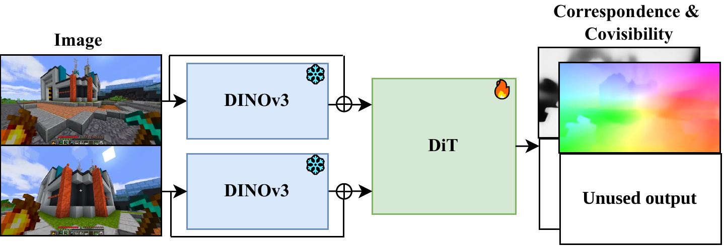
The figure hides the parts that make it work, so I traced the path with the numbers filled in from the paper's appendix and the code.
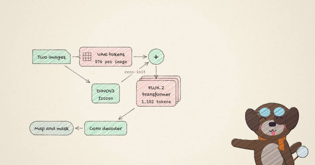
Each image is resized to 288 by 512. The frozen FLUX.2 VAE encodes it to a 36 by 64 grid of
32-channel latents, and every 2 by 2 neighbourhood is packed into one 128-dimensional token. That
gives 18 by 32, or 576 tokens per image. A frozen DINOv3 ViT-L/16 runs on the same image and
produces 1024-dimensional patch features on exactly the same 18 by 32 grid, because 16-pixel patches
and an 8x VAE with 2x2 packing land on the same stride. The code throws away the first five DINOv3
tokens, the class token and four registers (freematching/model.py:117).
The fusion is the simplest thing that could work. A linear layer maps 1024 DINOv3 dimensions to the transformer's 3,072, and its output is added to the image tokens right after FLUX's own input projection:
# freematching/vendor/model_flux2.py:847-859
hidden_states = self.x_embedder(hidden_states)
encoder_hidden_states = self.context_embedder(encoder_hidden_states)

if self.dino_proj is not None and dino_repre is not None:
    im_a_repre = self.dino_proj(dino_repre[0].to(hidden_states.dtype))
    im_b_repre = self.dino_proj(dino_repre[1].to(hidden_states.dtype))
    combined_dino_repre = torch.cat([im_a_repre, im_b_repre], dim=1)
    ...
    hidden_states = hidden_states + combined_dino_repre
That projection starts at exactly zero, weight and bias (freematching/model.py:29-32). On the
first training step the network is pure FLUX, and DINOv3 is let in only as fast as the gradient
finds it useful. This is the ControlNet trick, and it matters here because adding a random
3,072-wide vector to every token of a pretrained transformer would wreck its first few thousand
steps.
So to answer the question I came in with, which layers and which timesteps: DINOv3 contributes only its last hidden state, once, at the input. FLUX contributes all of itself. Nothing is read out of an intermediate layer.
The two 576-token sequences are concatenated into 1,152 tokens. FLUX.2's rotary position ids carry both the spatial position and which image a token belongs to, so attention can tell "same place in the other image" from "same place in this image". The transformer is FLUX.2-klein's, unchanged in shape: five double-stream blocks and twenty single-stream blocks, hidden size 3,072, 24 heads of 128, which I read from the checkpoint and the base model's config.
The text path is still there, and still fed. FLUX expects a prompt, so the code encodes an empty
string with the base model's Qwen3 text encoder, keeps two tokens of it, and passes them on every
call. The timestep input gets a constant. Then, of the 1,152 output tokens, the code keeps the
target's 576 (freematching/model.py:163-171), undoes the VAE's latent normalisation, unpacks them
back to a 32-channel 36 by 64 grid, and hands that to a small convolutional decoder.
The matching head is attention
There is no cost volume in FreeMatching, no argmax and no iteration. Every matcher I have worked with ends in one of those. RAFT refines a flow field over 12 or more recurrent updates. RoMa regresses a coarse warp from global matching and then refines it at several scales. FreeMatching makes one forward pass and regresses coordinates.
The matching happens inside the transformer. When a target token attends to the 576 source tokens, the attention weights are a softmax over similarities, which is the heatmap in the explorer above, computed in 24 heads at every one of 25 blocks. Whatever the network does with them, it writes into the target's tokens something that the decoder can read as two coordinates and a confidence. The attention is global by construction: no window, no pyramid, no starting guess.
The decoder (freematching/flow_decoder.py:73-161) is about 2.4M parameters of convolutions. Three
stages each upsample 2x, which takes 36 by 64 back to 288 by 512, and each stage adds its own
prediction of the coordinates and the mask to the upsampled previous one, so gradients reach the
coarse levels directly. A last block adds a correction squashed by a tanh, where flow_scale is 4 pixels expressed in
normalised coordinates, so it can move a prediction by at most 4 pixels:
# freematching/flow_decoder.py:149-159
flow_delta = self.flow_refine(torch.cat([x, flow], dim=1))
...
flow = flow + torch.tanh(flow_delta) * flow_scale
The output is three channels: normalised source coordinates for x and y, and a covisibility logit. I counted the released checkpoint's tensors from its safetensors header: 257 tensors and 3,881,134,812 parameters in BF16, of which 2,433,651 are the decoder and 3,148,800 the DINOv3 projection. Everything else is the fine-tuned FLUX transformer. The VAE, DINOv3 and the text encoder are fetched separately and stay frozen.
What "timestep" means when there is no noise
Since nothing is noised, the timestep is just a conditioning value. It sets the adaptive layer-norm
modulation in every block, the way a noise level would during generation. The paper says it is a
fixed . The code says 620: it is the default in both training scripts, in the inference
CLI and in both checkpoints' config.json, and the README calls 620 the value "matching the
original checkpoint evaluation". I would trust the code. The paper's value looks like it came from
an earlier draft.
Why does a constant timestep matter at all? Because FLUX's weights learned different jobs at different noise levels: near the clean end they sharpen detail, near the noisy end they lay out structure. Picking a mid-to-late value starts the fine-tune from the behaviour that already "knows" about object layout in a clean image. The paper does not ablate the choice, so that is my reading, not theirs.
Nine datasets, one Huber loss
Stage 1 is supervised. The mixture samples from nine sources, and the proportions in the paper's
Table 1 match configs/datasets.json exactly:
| Source | Share | What it teaches |
|---|---|---|
| ScanNet++ | 15% | indoor wide-baseline geometry |
| BlendedMVS | 10% | outdoor multi-view geometry |
| FlyingThings | 10% | synthetic flow, large motion |
| DynamicReplica | 10% | synthetic video, deforming people and animals |
| Spring | 5% | high-resolution flow |
| PointOdyssey | 5% | long synthetic tracks |
| FlyingChairs | 5% | the classic flow pretraining set |
| Video (theirs) | 20% | real non-rigid motion, pseudo-labelled |
| Blender (theirs) | 20% | clean multi-object rigid motion |
The two new sets carry 40% of the samples. The video set is 520k clips from ViPE, labelled by running AllTracker with 16-frame windows and four refinement iterations, then sampling frame pairs at varied gaps. This is how "tracked video" gets into a pairwise matcher: a dense point tracker labels pairs far apart in time, so the pairs have the large, non-rigid motion that flow datasets lack. The labels are a tracker's guesses, and they are not released. The README says the videos and trajectories cannot be distributed for size and copyright reasons, so you get the conversion code and have to source the clips yourself.
The Blender set is the clean counterweight: 360k pairs from Objaverse, two or three objects per scene, each object rotated by 30 to 50 degrees and rescaled by a factor of 0.8 to 1.2 between the two renders, with ground-truth flow from Cycles' motion vector pass and occlusion from alpha. Asset filtering throws out flat and needle-like meshes. It is the dataset I would have built for this task: independent motion of several objects, with exact labels.
Mixing pseudo-labels with exact labels is why the loss is Huber rather than L2. Its threshold
adapts: the code keeps an exponential moving average of the L1 error and sets the Huber delta to
twice that (train_flow_flux.py:672-674). Errors bigger than about twice the typical error are
penalised linearly, so a bad AllTracker label pulls on the gradient with a bounded force.
The paper's loss is a weighted sum of that Huber term on coordinates and an L2 term on the mask, with weights 10 and 0.2. The Stage 1 script computes something a little different:
# train_flow_flux.py:682
loss = loss_h * 10 + loss_mask * 0.33  + loss_grad * 1.0
The mask weight is 0.33, not 0.2, and there is a third term, a loss on the spatial gradient of the flow field that the paper does not mention at all. That term penalises the difference between the predicted and true flow gradients, so it pushes the predicted field to be as smooth, or as sharp, as the label. The training guide acknowledges the gap in its own words: it "retains its actual loss computation, including any gradient regularization". I do not think the gradient term changes the story. It is the kind of detail you want to know before trying to reproduce Table 6.
The teacher only has to fix small mistakes
Stage 1 sees no edited images. Stage 2 is where the model meets them, and the trick is how it gets a training signal with no ground-truth correspondence.
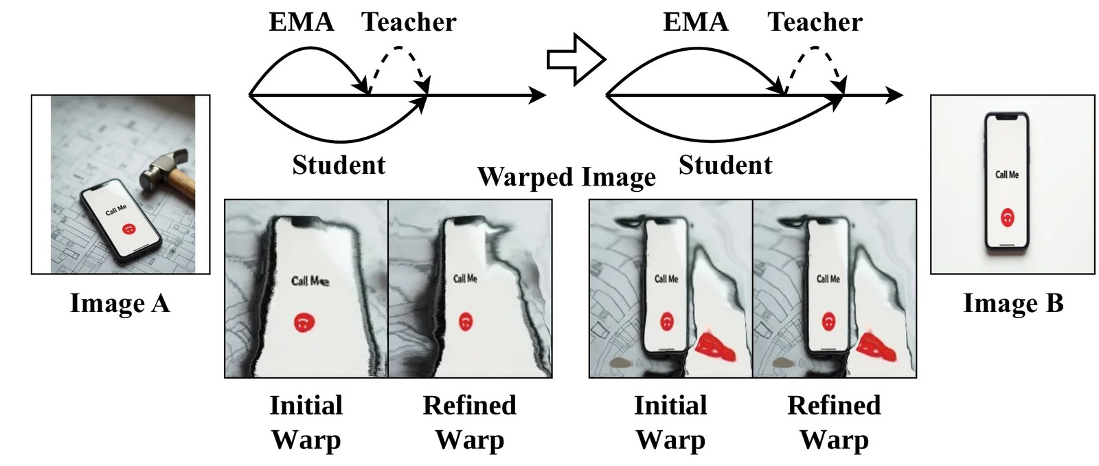
Three networks are involved. The student is the model being trained. An EMA copy of it, updated with decay 0.95 after every step, predicts an initial correspondence . The source is warped with , giving an intermediate image that should already look like the target, roughly.
A frozen teacher then matches the target against that intermediate image and returns a residual
map . The pseudo-label is the composition, : first follow the
teacher's small correction, then the EMA's big jump. The student is trained with the same adaptive
Huber loss toward , but only where the teacher's confidence passes 0.2 and the EMA's
covisibility passes 0.7 (train_flow_flux_roma.py:812-817), and its mask is pulled toward the
EMA's.
I like this design, and the reason is the paper's own title. A classical matcher fails on an edit because the two images are far apart. After the EMA's warp, they are not: the remaining error is local, a few pixels of misalignment around the edges of an object that is already in the right place. A matcher with spatio-temporal priors is good in exactly this regime. The paper puts the prior where it holds and lets the foundation model do the part where it does not.
Two details from the code. The teacher in the paper is RoMa. The teacher in the code is
romav2.RoMaV2 in its "fast" setting (freematching/training/teacher.py:130-157), and the
training guide says outright that this "backend name documents the implementation being
distributed; it is distinct from naming the RoMa baseline in the paper". And Stage 2 is not all
edited pairs: its loop runs three supervised updates for every weak one (--sup_steps_per_cycle 3 and
--weak_steps_per_cycle 1 in the guide's command), so about a quarter of what Stage 2 sees are IEG
pairs. The other three quarters keep the classical skills from eroding. The released Stage 2 model
is the EMA after 10,000 updates, starting from the Stage 1 checkpoint at step 275,000, with the
decoder frozen.
What the tables show
On edits
IEG-Bench is about 100 hard pairs drawn from the multi-reference subset of UNO's data, held out from the single-reference subset used for refinement. There is no ground truth, so quality is measured by reconstruction: warp the source with the predicted map and compare it with the target inside the covisible region.
| Model | Ref-MSE ↓ | LPIPS ↓ | SigLIP 2 ↑ | DINOv3 ↑ |
|---|---|---|---|---|
| Identity (no warp) | 23.65 | 81.97 | 86.67 | 52.38 |
| SEA-RAFT | 18.49 | 72.45 | 85.18 | 58.14 |
| UniMatch | 11.07 | 58.42 | 87.86 | 66.35 |
| RoMa | 8.08 | 48.91 | 87.73 | 70.15 |
| UFM | 10.41 | 53.05 | 86.97 | 66.77 |
| FreeMatching | 6.22 | 45.41 | 90.77 | 80.01 |
FreeMatching wins every column, and by a lot on the two that move most: Ref-MSE is about 23% below RoMa's and the DINOv3 score is nearly ten points higher. The qualitative figure is more convincing than the numbers. In row after row, the flow models produce silhouettes filled with the wrong content, RoMa and UFM tear the object into pieces, and FreeMatching gets the whole object.
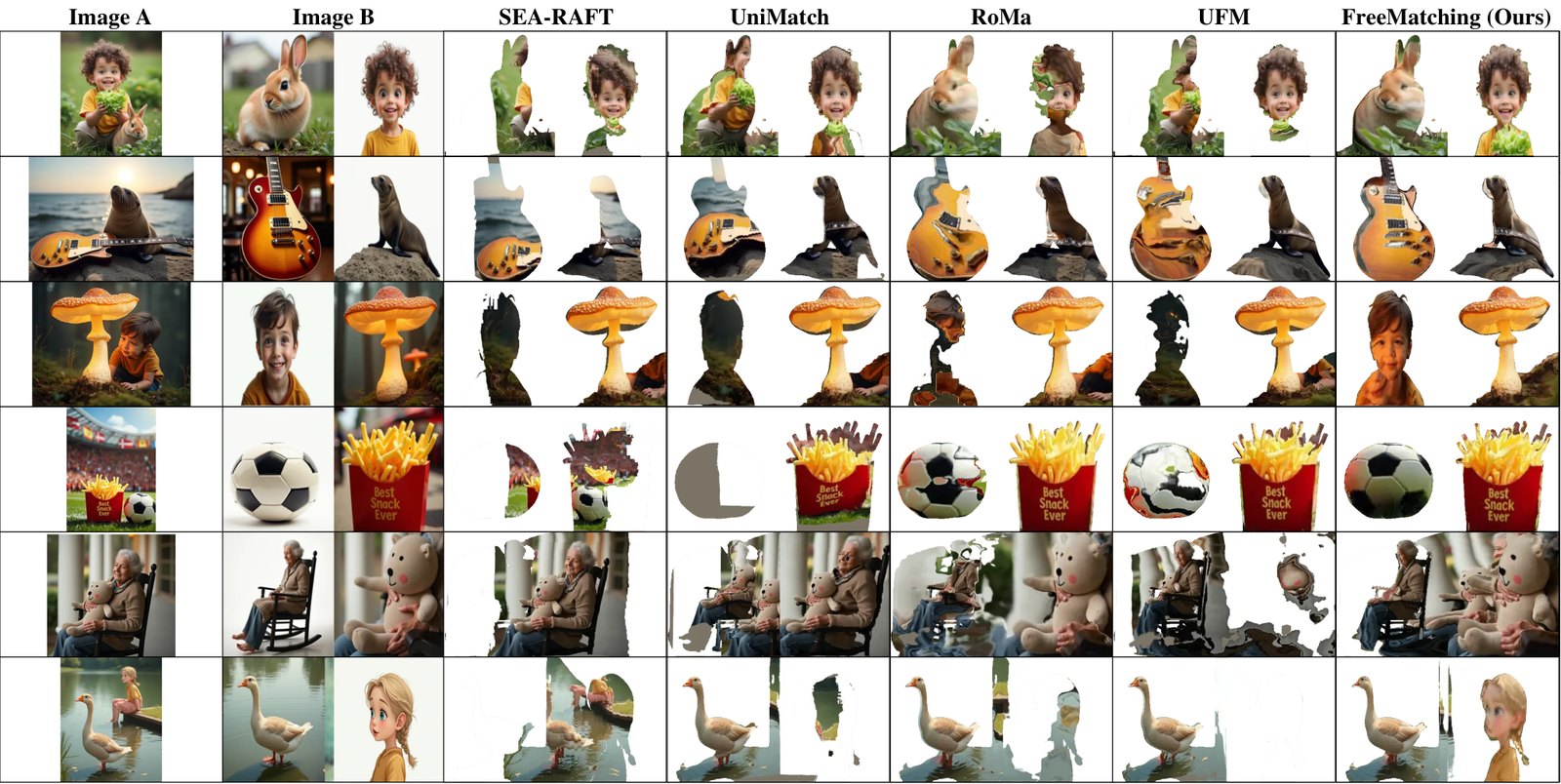
Table 6 builds the system one component at a time, scored by the DINOv3 metric: a randomly initialised DiT trained on classical data gets 67.31, FLUX initialisation brings it to 69.28, DINOv3 inputs to 72.76, the video and Blender data to 76.52, and refinement to 80.01. Each step is worth two to four points, and the two foundation models together are worth less than the new data plus refinement.
The paper's human study points the same way: ten raters scored warps blind on a 0 to 3 scale, and the mean opinion scores were 2.25 for FreeMatching, 1.39 for RoMa, 1.13 for UFM and 0.49 for SEA-RAFT. Their Pearson correlation between the human ratings and the DINOv3 score is , though the paper does not say whether that is computed per pair or per method.
Things I would want a reviewer to ask
The DINOv3 score is computed with DINOv3, and FreeMatching is the only model that is given DINOv3 features as input. A model whose warps look good to DINOv3 has an obvious advantage on that column, and Table 6, the ablation, is scored only with it. The paper does answer this in a second comparison, Table 5, which uses DINOv2 and OpenCLIP instead. There, FreeMatching scores 54.31 and 70.56 against UFM's 39.65 and 56.48 and RoMa's 47.14 and 61.18. The lead survives a change of judge, so I would not dismiss the main table on this ground. I would not use the ablation's 2-to-4-point steps to argue that one component matters more than another, either.
The reference masks were seeded by FreeMatching. The appendix says so: "FreeMatching predictions provide initial candidates", which human annotators then screened, edited and froze before applying them to every method. The finalisation by hand makes this less of a problem than it sounds, and Full-MSE, which uses no mask at all, also favours FreeMatching (10.99 against 13.48 and 16.57). Still, a mask drawn around where your own model found a counterpart is a mask that will never penalise you for the regions you missed.
The teacher is a matcher it is compared against. FreeMatching after Stage 1 scores a Ref-MSE of 8.08 in Table 10, the same 8.08 RoMa scores off the shelf in Table 4. All of the measured lead on that metric arrives in Stage 2, the stage in which a RoMa-family model labels the pairs. It is a legitimate method, distillation from a strong local matcher wrapped around a global one. It also means a better teacher would probably lift the student, and the paper's "beyond priors" framing undersells how much the prior-based model still contributes. One more number from Table 10 belongs here: refining on unlabelled flow pairs instead of edits already brings Ref-MSE from 8.08 to 7.26. About 44% of the Stage 2 gain comes from running the self-training loop at all, on any data.
Table 5 also fine-tunes UFM and RoMa with the same 10k-step IEG adaptation, which is the fairest comparison in the paper. The odd thing is that RoMa gets worse from it (8.08 to 9.70 Ref-MSE), and UFM gets better (10.41 to 8.55). The paper does not comment. It suggests the adaptation recipe was tuned for FreeMatching, which would be normal and is worth knowing.
On classical benchmarks
This is where I would read the paper most carefully. The headline claim is that a single model "achieves performance competitive with SOTA methods on classical optical flow and dense matching benchmarks".
The first thing I noticed is that the UFM and RoMa rows in Tables 2 and 3 are not the published models. Their numbers are identical, to the last digit, to the rows labelled "UFM (10k-IEG)" and "RoMa (10k-IEG)" in Table 9: the versions fine-tuned on edited images. The text says it, "lower EPE than the similarly adapted UFM and RoMa variants", but the table captions do not, and off-the-shelf numbers for those two are not given anywhere. For a reader comparing against what they would download, the right comparison is missing.
On dense matching it is a real win. ScanNet-1500 EPE is 8.56 against 12.03 for both adapted baselines, and ETH3D is 10.23 against RoMa's 11.26. Pose AUC is a tie with RoMa, which comes out slightly ahead at 20 degrees on both sets, 78.61 against 78.23 on ETH3D and 70.90 against 70.03 on ScanNet.
On optical flow it is not competitive with the flow models, and the paper's own text half-admits it ("UniMatch achieves the lowest EPE among the methods shown"):
| Method | Sintel clean EPE | Sintel final EPE | KITTI-2015 EPE |
|---|---|---|---|
| SEA-RAFT | 0.43 | 0.81 | 1.97 |
| UniMatch | 0.40 | 0.75 | 1.52 |
| UFM (10k-IEG) | 0.92 | 1.48 | 4.75 |
| FreeMatching | 1.05 | 1.36 | 4.95 |
FreeMatching's Sintel clean EPE is about 2.6 times UniMatch's, and its KITTI EPE about 3.3 times. It is in the same band as the adapted generalist UFM, which is a fair peer, and far from the flow specialists. I would call that "retains usable flow", not "competitive with SOTA".
Several things I could not check would matter for the flow numbers. The paper says the authors "recompute the results ourselves" on covisible regions only, which is not the official protocol; it does not say which checkpoint of each baseline was used; and EPEs as low as SEA-RAFT's 0.43 on Sintel usually come from a checkpoint that saw Sintel in training, which would make those rows in-domain while FreeMatching's are zero-shot. It also does not say at what resolution each baseline ran or how many refinement iterations RAFT-family models were given at test time. FreeMatching itself works at 288 by 512, which is less than a third of a Sintel frame's pixels (1024 by 436) and less than a third of KITTI's. Sub-pixel EPE at the original resolution, from a prediction made on a smaller grid, is fighting with one hand tied. No evaluation code is released, so none of this can be read off the repo.
And the baselines the brief asked me about mostly are not there. RAFT appears only through SEA-RAFT. CoTracker is cited as background for tracked video, not compared; AllTracker is a data labeller, not a baseline. DUSt3R and VGGT appear in related work only, MASt3R not at all. DIFT is not compared either. The one semantic matcher shown is SD-DINO, in a single qualitative example in the appendix, where it is run with text prompts and loses. For an edit-matching paper the missing semantic-correspondence comparison is the gap I would most like to see filled.
What a pair costs
The paper is upfront that it is slow, and the appendix measures it: on one H20 at 288 by 512 with batch 1, FreeMatching takes 121.9 ms a pair and peaks at 15.18 GiB of allocated memory. UFM takes 51.3 ms and 2.35 GiB, and RoMa 102.5 ms and 2.58 GiB. So it is about 2.4 times slower than UFM and uses about 6.5 times its memory, at a resolution most flow benchmarks would call small.
I tried to account for the 15.18 GiB from the files. The checkpoint is 7,762,299,928 bytes. DINOv3 ViT-L/16 is 1.21 GB in FP32 on the hub, about 0.6 GB once the loader casts it to BF16. The VAE is another 0.17 GB at most. Together, about 7.9 GiB of weights touched per forward pass. Attention over 1,152 tokens and a 96-channel decoder at 288 by 512 cost tens of megabytes, not gigabytes. I can't say what the other half of the peak is; the profiling script is not in the repo.
One thing the released loader does that the paper does not mention: to get the empty-prompt
embedding, build_model_stack loads FLUX.2-klein's Qwen3 text encoder, 8,044,981,992 bytes of
BF16, onto the GPU alongside everything else (freematching/model.py:41-80), encodes the empty
string once, and deletes it. During startup that is roughly 15.4 GiB of weights resident at once.
The paper says the embeddings are cached. In the released code they are cached only after that
first load, so if you are trying to fit this on a 16 GB card, precompute the two-token embedding
once and skip the text encoder entirely.
Resolution is the other cost. Every image is resized to 288 by 512, and the code requires multiples of 16. Attention cost grows with the square of the token count, so doubling each side to 576 by 1024 quadruples the tokens to 2,304 per image and multiplies the attention work by sixteen. The model was trained only at 288 by 512, too, so going higher is an extrapolation in both cost and accuracy.
Training is the cost most people will not pay. The paper reports 768 A100 GPU-hours for 150k Stage 1 updates and 80 for Stage 2, on 16 A100s. Then it adds that these figures describe "the original training configuration reported in the rebuttal", not the released run. The released Stage 1 checkpoint is at step 275,000, nearly twice as many. If the rate held, that is around 1,400 A100 hours, a figure I computed and the paper does not give. And the video data has to be re-collected and re-tracked by you.
Where I would use it
As a metric, today. The paper's last application is the one I find most immediately useful: warp the reference onto an edited image and look at the per-patch DINOv3 similarity inside the covisible region. Global scores like a CLIP or DINO similarity on the whole image average away a changed logo or a missing stripe. A spatial map does not.
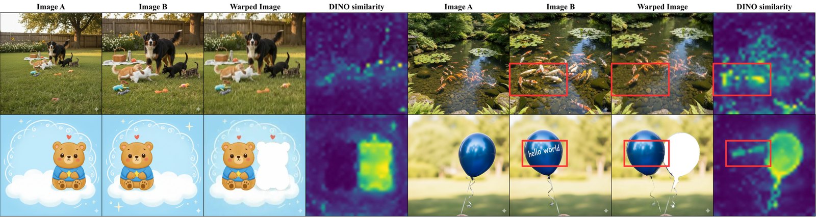
For a team evaluating subject-driven generation or image editing models, that is a real tool: it says not only that identity drifted, but where. At 121.9 ms a pair it is cheap enough for an eval set of thousands.
As an optical flow estimator, no. The specialists are two to three times more accurate on Sintel and KITTI, faster, and run at the resolution you have. As a wide-baseline matcher for pose, it ties RoMa at about six times the memory. If you are already computing correspondences for dense 3D tracking or reconstruction, this is not the model to swap in.
Then there is the toy's second star. FreeMatching regresses one answer per pixel. When an edit duplicates an object, which image generators do readily, a single-answer regressor has to pick one copy or, like the soft-argmax in the explorer, blur toward the middle. The paper knows this: Appendix F sketches a diffusion version that would sample one hypothesis per noise seed, then notes that "all reported experiments use the efficient single-pass regression model". A model built from a diffusion transformer, running with the diffusion switched off, would be the obvious place to put it back.
The broader lesson is the one that keeps coming up on this site. Marigold V2 turned a 20B image-editing transformer into a depth estimator. RelateAnything built a scene-graph model on DINOv3. Here a 4B image generator, with DINOv3 bolted onto its input and all of its weights fine-tuned, becomes a matcher. The generative pretraining is doing the work that used to be done by hand-designed cost volumes. The bill comes in memory, and in the fact that the result runs at a resolution its pretraining chose.
How I checked
I read v1 of the paper in arXiv's HTML and its LaTeX source, and took Figures 1 to 5 from the
source PDFs. I shallow-cloned luping-liu/FreeMatching (commit 20add551, 8 October 2026) and
read the model, decoder, teacher, both training scripts, the dataset config and the docs; I did not
run any of it. The parameter counts are from the safetensors header of the Stage 2 checkpoint, read
with an HTTP range request, and the base model's shape is from its transformer/config.json on
Hugging Face. The weight sizes for DINOv3, the VAE and the Qwen3 text encoder are the file sizes the
Hugging Face API lists. Everything in the "what the tables show" section is the paper's own numbers;
the relative figures (23%, 2.6 and 3.3 times, 44%, 2.4 and 6.5 times, about 1,400 GPU-hours) are my
arithmetic on them. The explorer is toy data and says so. I could not check anything about how the
baselines were evaluated, because no evaluation code is released.