Land or Water?: reading a world map out of 16,200 one-word answers

2026-10-06 · 20 min · explainer · llm · evaluation · benchmarks · interpretability · world-models

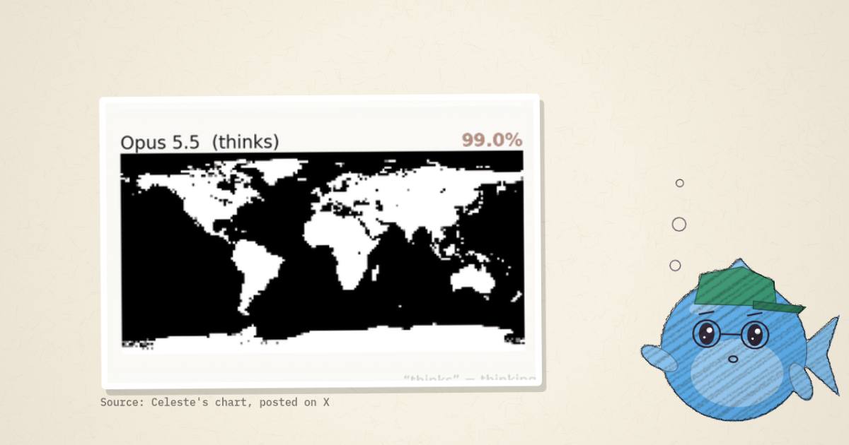
Andrej Karpathy put it in one post: "Simply ask an LLM 'Land or Water?' and give it a latitude and longitude coordinate as text. Ask 16,200 times, plot as image. The models know. From compressing the internet." He was quote-posting a chart by Celeste (@celestepoasts) of twelve Claude models drawing the Earth, one point at a time.

The eval is older than the chart. It comes from Henry (@arithmoquine), whose August 2025 post How Does A Blind Model See The Earth? set out the method and ran it on about forty models. A day after Karpathy's post, Favio Vazquez published an open reproduction on CPU-only open models, with every raw answer committed as CSV. That repo is what made this article checkable. I could score maps myself instead of trusting the labels on a picture.

This piece covers what the eval does mechanically, what the published maps show once you score them yourself, where the errors actually fall, what it costs, and why a model trained only on text can answer at all.

Labels: measured means I computed it from a committed file or a published image. Reported is the publisher's number, not re-run. Reasoned is my arithmetic on the other two.

The method, in four lines

Henry's procedure, quoted from his post:

Sample latitude/longitude pairs evenly across the globe.
For each one, ask an instruct-tuned model: "If this location is over land, say 'Land'. If this location is over water, say 'Water'. Do not say anything else. x° S, y° W".
Read the logprobs of the tokens "Land" and "Water" at the first answer position, and softmax the two.
Paint each probability as one pixel of an equirectangular map.

Step 3 is the useful part. You never parse the model's text. You read one forward pass's next-token distribution and keep two entries of it:

P(\text{Land}) = \frac{e^{\ell_L}}{e^{\ell_L} + e^{\ell_W}}

Here $\ell_L$ and $\ell_W$ are the log-probabilities the model assigns to the first token of "Land" and of "Water". Every other token gets thrown away. Henry notes that tokenization doesn't matter much: if "Land" splits into "La" + "nd", you look for "La". It's the same single-pass, named-candidate readout that SGLang's /v1/score endpoint exposes, and that decision models like Jev are built around. The site has covered both.

When an API doesn't return logprobs, Henry sampled each point several times at temperature 1 and used the vote share. He used four samples for Claude and Gemini ("n=4 approximation"), one for Opus because of price, and eight for one Gemini run. He reports that eight samples "do not smooth out the distribution".

Why one point per prompt instead of "draw me a map as SVG"? Henry's answer: "whatever caricature the model spits out upon request would have little to do with its actual geographical knowledge." A per-coordinate query asks the model to recall a fact. A drawing request asks it to perform one. Those can come apart.

The grid: where 16,200 comes from

Celeste's chart subtitle says "at every 2° of the globe · 16,200 points". The open reproduction pins the grid exactly: latitudes 89 down to −89 and longitudes −179 to 179, both in steps of 2 (run.json: "lats": [89, -89, 2], "lons": [-179, 179, 2]). That's 90 rows × 180 columns = 16,200 cell centres (measured, the answer key has 16,200 rows). Halving the step to 1° gives 180 × 360 = 64,800 prompts (reasoned). Henry calls this "the Tyranny Of Power Laws": twice the sharpness costs four times the queries.

Two scoring details matter more than they look:

Area weighting. In an equirectangular grid, a cell at 80° covers about a sixth of the ground a cell at the equator does. Both Celeste's chart and the reproduction weight each point by $\cos(\text{latitude})$ . Without that weighting, Antarctica and the Arctic would count as heavily as the tropics.
The always-"Water" floor. On this grid, 5,379 of 16,200 points are land in the Natural Earth 1:10m answer key. So answering "Water" every time scores 66.8% plain and 71.1% area-weighted (measured from the repo's data/landmask_ne10m_land_v5.1.1.csv, which matches the repo's stated floor). Any score below 71% knows less than a constant.

What the Claude chart shows

A four-by-four grid of black-and-white world maps. The first panel is the real Earth. The rest are Claude models from Sonnet 4.5 to Opus 5.5, each with an area-weighted accuracy in orange: Sonnet 4.5 60.5% shows land almost everywhere, Haiku 4.5 81.3% is mostly black with grey noise, Opus 4.5 82.6% has blob continents, the 4.6 to 5 generation sit between 89.1% and 92.5% with recognisable continents, and the thinking runs of Fable 5, Fable 5.1 and Opus 5.5 reach 97.8%, 98.2% and 99.0% with sharp coastlines. The bottom row shows no-thinking runs at 95.9%, 96.5% and 96.4%. — Celeste's full chart: the real Earth, twelve Claude models, and three no-thinking runs, each at 16,200 points on a 2° grid, white = Land. The orange specks on 'Fable 5, no thinking' are points where, by her account, the model couldn't be stopped from thinking. Accuracies are hers, area-weighted against a 1-km land mask. (Celeste, @celestepoasts, 'here's no thinking' chart posted on X.)

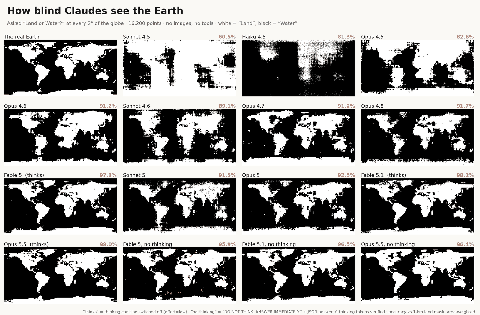
The published numbers (reported, from the chart):

model	area-weighted	model	area-weighted
Sonnet 4.5	60.5%	Opus 4.8	91.7%
Haiku 4.5	81.3%	Sonnet 5	91.5%
Opus 4.5	82.6%	Opus 5	92.5%
Opus 4.6	91.2%	Fable 5 (thinks)	97.8%
Sonnet 4.6	89.1%	Fable 5.1 (thinks)	98.2%
Opus 4.7	91.2%	Opus 5.5 (thinks)	99.0%

Three things stand out once you put the 71.1% floor next to the table:

Sonnet 4.5 is below the floor. At 60.5% it does worse than answering "Water" everywhere, because it says "Land" at most points on the map. That's a bias problem as much as a knowledge problem: its map still has a dark ocean down the left side.
Haiku 4.5 at 81.3% is mostly "Water" with a grey cloud over Eurasia. Its score is about ten points above the floor, and that's all a constant-plus-noise strategy can earn.
Thinking is worth about 2.6 points at the top. Opus 5.5 scores 99.0% with thinking and 96.4% with Celeste's "DO NOT THINK. ANSWER IMMEDIATELY." prompt (reported). Fable 5 goes from 95.9% to 97.8%. The single-chart version of the Opus 5.5 run says "thinks (effort=low), 2 samples/point".

Celeste hasn't published her prompt or code. The exact wording, the thinking budget, how two disagreeing samples were combined, and which 1-km mask she used are all unverified. Her footnote says only "accuracy vs 1-km land mask, area-weighted".

Reading the chart back, cell by cell

A chart with 16,200 cells per panel holds its own data. Each panel in the 2700 × 1769 PNG is 635 × 317 pixels, which works out to about 3.5 pixels per grid cell. I sampled the centre of every cell in every panel and scored the result against the reproduction's Natural Earth key. The digitized maps reproduce Celeste's stated accuracies to within half a point for fourteen of fifteen panels, and to 0.9 for the worst: Opus 5.5 (thinks) 99.0 against 99.0, Opus 5 92.6 against 92.5, Sonnet 4.5 59.6 against 60.5. Her "real Earth" panel agrees with the Natural Earth key at 99.7% area-weighted (measured). That's close enough to ask the question the chart can't answer by eye: where are the wrong points?

I define a point as coastal if any of its eight neighbours on the 2° grid has the opposite true answer. That ring holds 3,540 of the 16,200 points: 21.9%, call it 22% (measured).

model	wrong points	share on the coastal ring	error rate, coastal	error rate, inland/open sea
Sonnet 4.5	7,005	26%	51.7%	40.9%
Opus 4.5	3,787	40%	43.3%	17.8%
Opus 5	1,473	73%	30.3%	3.2%
Opus 5.5, no thinking	868	83%	20.3%	1.2%
Opus 5.5, thinking	292	82%	6.8%	0.4%

(measured, digitized from Celeste's chart, scored against Natural Earth 1:10m.)

As models improve, their errors pile up on the coast. A weak model is wrong everywhere. Its errors land on the coastal ring at about the ring's own share, which is what noise looks like. A strong model is wrong almost only where land meets water. At that point the eval mostly measures coastline sharpness at 2° resolution, a scale where "is this cell centre land?" is close to a coin flip for any honest observer.

Some of those coastal "errors" aren't errors. The Natural Earth land polygons include inland lakes as land. On this grid, 37 points fall inside a lake polygon, and the key marks all 37 as land. Opus 5.5 (thinking) answers "Water" at 17 of them: Superior, Michigan, Huron, Victoria, Ladoga and Baikal among them (measured). That's 6% of its 292 errors where the model is arguably right and the key is wrong. A reply under Celeste's chart caught this by eye: "The latest claude's get the great lakes correct and 'the real earth' gets them wrong." So at 99%, the remaining point is partly a disagreement about what "over water" means.

Play with the grid

The widget below holds nine of these maps as bits: the answer key, the open reproduction's Gemma 4 26B-A4B run, and seven of Celeste's Claude panels as digitized above. The grid slider thins the grid by keeping every k-th point in each direction. That's exactly the set of prompts a coarser run would send, though here it's read back from the 2° answers rather than re-run. "Errors" view splits wrong points into coastal and inland. The samples control multiplies the call count, the way Henry's n=4 and Celeste's two samples did.

land-or-water · 2° grid · 16,200 prompts

grid step: 2° (90 x 180)

samples per point

API calls: 16,200
prompt tokens: ~842,400
area-weighted: 99.0% (all Water 71.1%)
wrong points: 292 (82% coastal)

Source: Celeste chart. A coarser step keeps every point of the 2° answers in each direction, which is the set of prompts a coarser run would send; it is read back, not re-run. Prompt tokens assume about 52 per call, the Gemma 4 run's measured average; thinking tokens, which the Claude runs spend, are not counted.

Thinning the grid shows that the 16,200 points buy the picture, not the score. Opus 5.5 (thinking) scores 99.0% on all 16,200 points, 99.1% on the 1,800-point 6° grid, and 99.6% on the 648-point 10° grid (measured with the widget's own subsampling, mirrored in Python). Accuracy is a proportion. A proportion's estimate barely depends on how many points you take once you have a few hundred. What 25 times more prompts buys is the coastline: Florida, the Red Sea, the gap between Sumatra and Malaya. If you want a leaderboard number, 648 prompts gets it to within a point. If you want to see what the model knows, you need the full grid.

What it costs

The eval is cheap per point and expensive in count.

Prompt size. The open reproduction's Gemma 4 run evaluated 846,900 prompt tokens over 16,200 points, about 52 tokens per prompt including the chat template (measured from run.json). The answer is a single token read from the logits, so there's no generation cost when logprobs are available.
Wall clock on CPU. That same run took 2,930 seconds, 0.181 s per point, on 60 threads of an AMD EPYC 9R14 with 8-bit weights. That's about 49 minutes for the full map (reported, from the run file).
Sampling multiplies it. Without logprobs, the Claude runs pay per sample. Henry's n=4 at 2° is 64,800 calls. Celeste's Opus 5.5 at two samples per point is 32,400 calls, and each one is allowed to think at low effort (reasoned). The thinking tokens dominate the bill and aren't published, so I won't put a price on her run.
One price that was published. Henry's September 2026 Jev rerun was financed by a friend for "$7" (reported). The post doesn't break down how many points or questions that covered. His continent map is labelled "1° grid · one 8-way question per point", so it's at least 64,800 questions.

A land-probability heat map of the world from TypeSafe's jev-1.13.0, blue for water and green for land, with recognisable but blobby continents, a horizontal artefact line along the equator, and a solid green band along the bottom for Antarctica. — The same eval on Jev, a decision model that returns calibrated probabilities over typed answers in one pass, so P(Land) comes out directly instead of being sampled. Henry says its grasp of the globe is 'on par with some of the best models a year ago'. (Henry, @arithmoquine, post on X, typesafe/jev-1.13.0.)

What the open models show, and the minus-sign trap

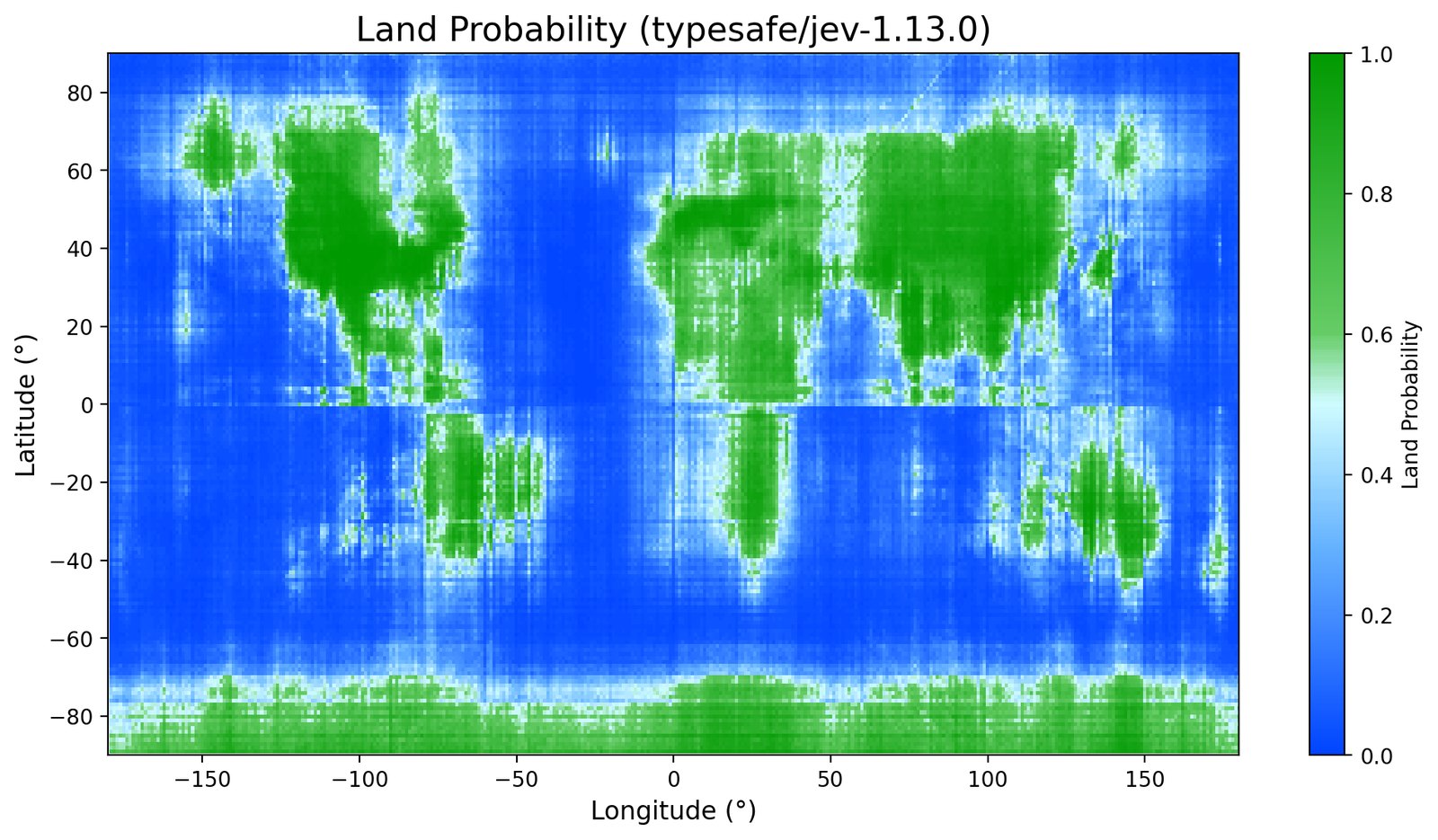
Henry's original survey is mostly open models read through real logprobs. His Qwen 2.5 ladder is the cleanest scaling picture. At 0.5B the model says land everywhere. At 1.5B "the northeastern quadrant has stuff going on". At 7B the continents split. By 72B the shape is right.

A blue-and-green land probability map from Qwen2.5-7B-Instruct: one large green blob over Eurasia and Africa's north, a smaller blob over North America, a small one where Australia should be, and blue elsewhere. — Qwen2.5-7B-Instruct: 'Proto-America and Proto-Oceania have split from Proto-Eurasia'. Henry points at the smooth boundaries as evidence against rote memorisation of individual places. (Henry, 'How Does A Blind Model See The Earth?', Outside Text.)

A land probability map from Llama-3.1-405B-Instruct with recognisable continents, a clear Mediterranean, Red Sea and Gulf of Mexico, and a green Antarctic band. — Llama-3.1-405B-Instruct, which Henry calls the 'best rendition of the Global West so far' and attributes tentatively to its being the only confirmed dense model of its size. (Henry, 'How Does A Blind Model See The Earth?', Outside Text.)

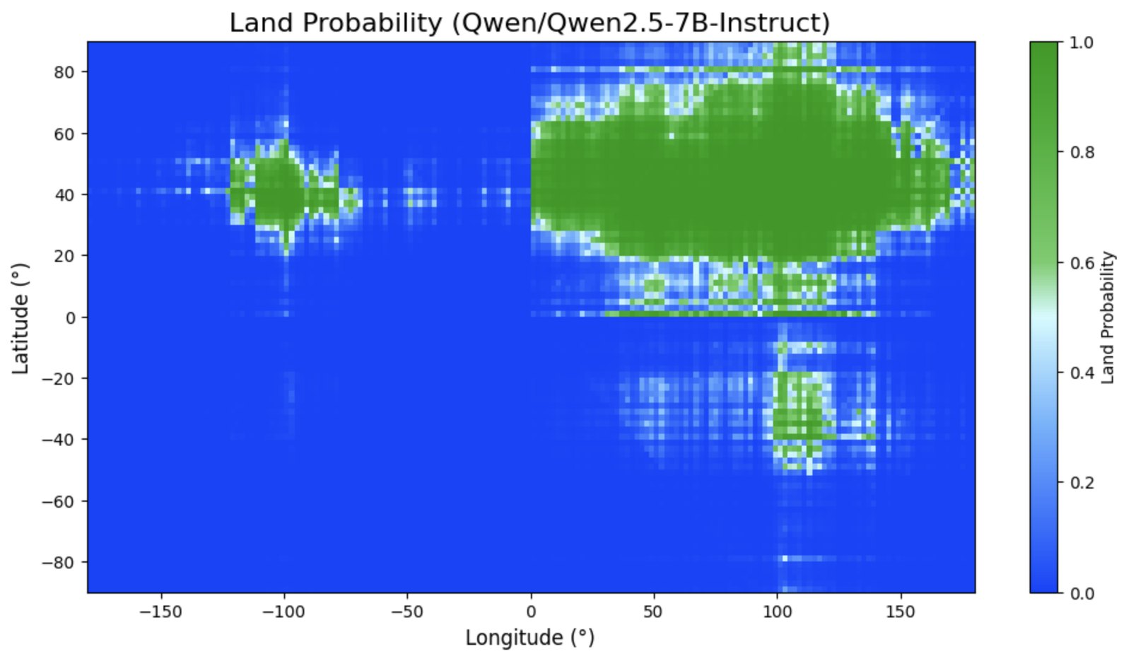
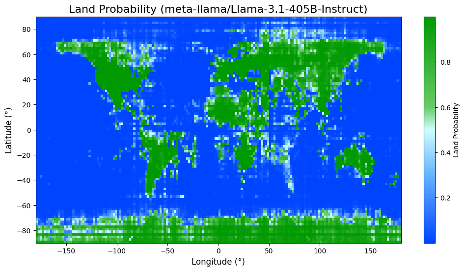
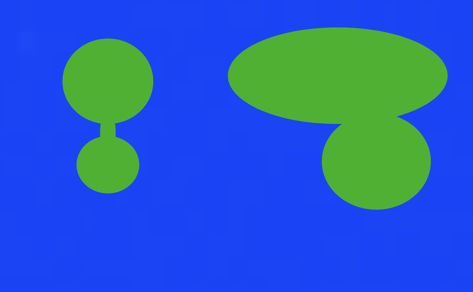
Henry also sketches what he calls an "Ideal Platonic Primitive Representation of The Globe": the shape that keeps showing up across mid-sized models. It's two lobes in the west and one large mass with a southern bulb in the east.

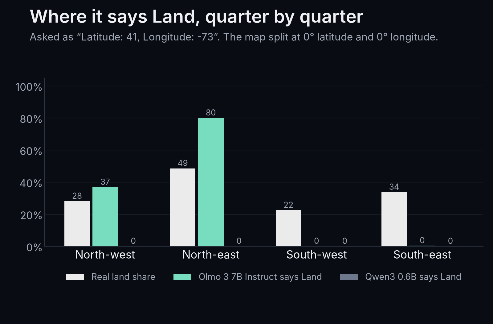
A hand-drawn schematic in green on blue: on the left, a round lobe joined by a thin neck to a smaller round lobe below it; on the right, a wide oval with a large round lobe hanging beneath it. — Henry's sketch of the primitive globe mid-sized models seem to converge on, roughly the Americas on the left and Eurasia over Africa on the right. A drawing of his hypothesis, not data. (Henry, 'How Does A Blind Model See The Earth?', Outside Text.)

The open reproduction tried to rerun this on hardware anyone can rent and hit a trap Henry's phrasing happens to avoid. Ask with signed decimals (Latitude: 41, Longitude: -73) and small models answer the minus sign, not the place. Olmo 3 7B Instruct said "Land" at 80% of the points where both numbers are positive and at 0% of the south-west quadrant (measured from runs/full/olmo-3-7b-instruct-signed.csv: north-east 0.800, south-west 0.000). Qwen3 0.6B said "Water" at 16,199 of 16,200 points (reported; I count 0.0% Land too). The repo says quadrant alone explains 71% of the variation in Olmo's answers, against 4% for the real map (reported).

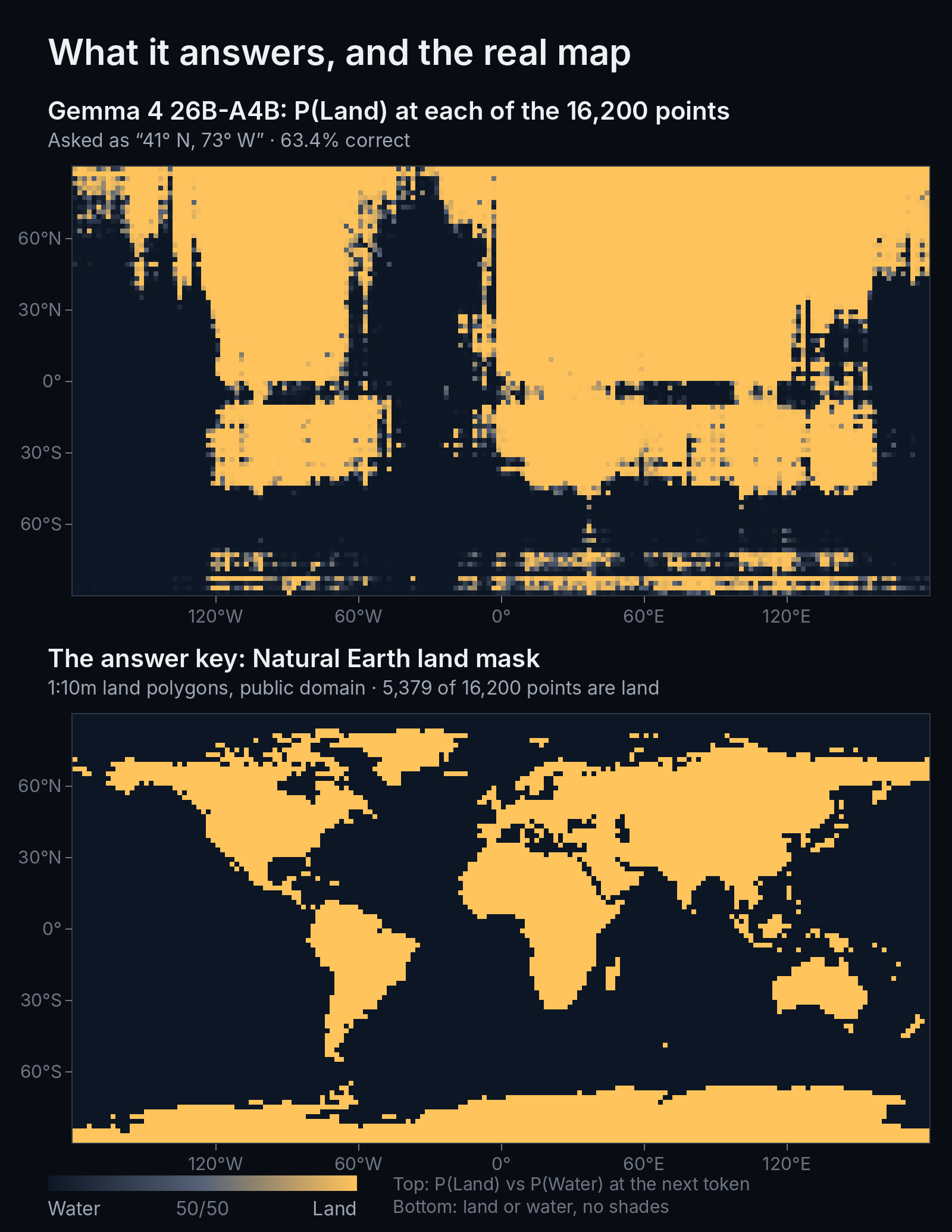
A bar chart titled 'Where it says Land, quarter by quarter' with four groups, North-west, North-east, South-west and South-east. Real land share is 28, 49, 22 and 34 percent. Olmo 3 7B Instruct says Land at 37, 80, 0 and 0 percent. Qwen3 0.6B says Land at 0 in all four. — Asked with signed decimals, Olmo 3 7B tracks the signs of the numbers rather than the geography. (Favio Vazquez, land-or-water repository, quadrants_f1.png, CC BY 4.0.)

Its best run, Gemma 4 26B-A4B with Henry's degree-and-hemisphere phrasing, draws real continents. It still scores 68.7% area-weighted, below the 71.1% floor, with an AUC of 0.755 (measured: I recompute 68.7% and 0.7555 from the committed CSV, thresholding P(Land) at 0.5). AUC is the useful number here. It asks whether a random land point gets a higher P(Land) than a random water point, so it ignores the model's bias toward one word. Gemma ranks land above water three times in four. It just says "Land" at 51% of points when only a third are land.

Two stacked maps on a dark background. Top: Gemma 4 26B-A4B's answers in yellow, with blocky but recognisable Americas, Africa and Eurasia, plus extra land across the North Pacific and a horizontal band. Bottom: the Natural Earth answer key, with 5,379 of 16,200 points marked land. — The best open model a CPU box can run, against the answer key: the outline of the world, not its coastline. (Favio Vazquez, land-or-water repository, final_vs_truth.png, CC BY 4.0.)

The repo is also honest about a gap I can't close. Its Qwen2.5 7B run "never matched the reference write-up's picture of that model", and nobody knows why yet. Prompt format, chat template and quantization all move these maps. The repo found a missing start-of-text token that took Gemma's AUC from 0.67 to 0.76 once fixed (reported). So treat any single map as one setting of many knobs.

Why it works: space is a straight line in the activations

"The models know" is a claim about internal representations, and someone has measured it. Wes Gurnee and Max Tegmark's Language Models Represent Space and Time (2023) ran 39,585 world place names through base Llama-2 models: cities, landmarks, lakes, and so on. They saved the residual-stream activation on each name's last token and fit a linear ridge regression from that vector to the place's true latitude and longitude:

\hat{W} = \arg\min_W \lVert Y - AW \rVert_2^2 + \lambda \lVert W \rVert_2^2

$A$ is the $n \times d_{\text{model}}$ matrix of activations, $Y$ holds the $n$ true (latitude, longitude) pairs, and $\lambda$ is the ridge penalty. If a single matrix multiply recovers coordinates for places the probe never saw, then position is laid out along directions in the model's activation space.

It does. On held-out places, Llama-2-70b's layer-50 activations projected onto the two learned directions draw a recognisable world:

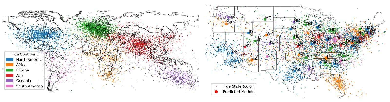
Two scatter plots. Left: thousands of held-out world places plotted at their probe-predicted latitude and longitude over a world outline, coloured by true continent; North America, Europe, Asia, Africa, Oceania and South America form distinct clouds roughly in the right places. Right: US places at predicted positions over a state map, coloured by state, with each state's median prediction labelled near its true location. — Each point is a held-out place name's layer-50 activation in Llama-2-70b, projected onto the learned latitude and longitude directions. (Gurnee and Tegmark, 'Language Models Represent Space and Time', Figure 1, arXiv 2310.02207.)

Two results from the paper explain the eval's scaling pictures:

The representation builds through the first half of the network and then plateaus, and bigger models encode it better. Llama-2 (2T training tokens) beats Pythia (300B) by a wide margin. The authors suspect training-corpus size is the reason (reported).
It's linear. A one-hidden-layer MLP probe with 256 units can bend the read-out any way it likes, and it buys almost nothing. For Llama-2-70b on world places, linear R² is 0.911 and MLP R² is 0.926 (reported, Table 2). In the NYC dataset the MLP is worse.

Six line charts of test R squared against relative model depth from 0 to 1, one per dataset: World Map, USA Map, NYC Map, Historical Figures, Entertainment, Headlines. Llama-2-70b, 13b and 7b are solid lines at the top; Pythia models from 160m to 6.9b are dashed lines lower down. Most curves rise over the first half of depth and then flatten. — Out-of-sample R² for linear probes at every layer of every model: rising through the first half of depth, then flat, with Llama-2 well above Pythia. (Gurnee and Tegmark, 'Language Models Represent Space and Time', Figure 2, arXiv 2310.02207.)

probe R² · straight line vs MLP · 60% depth

linear ridge probeMLP probe, 256 unitsnumber = MLP minus linear

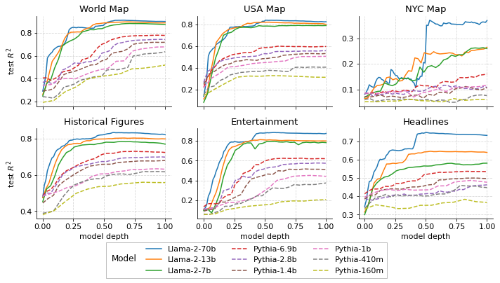
Out-of-sample R² from Table 2 of Gurnee and Tegmark (2023). World, USA and NYC are the place datasets; the other three are time. Values copied from the paper, not re-run.

Here is the static version of what the widget shows. For world places, the MLP minus linear R² is +0.016 at 7B, +0.020 at 13B and +0.015 at 70B. For NYC it's −0.015, −0.007 and −0.047. For headlines it's −0.097 at 7B (reasoned, differences of the Table 2 entries). A straight line in activation space captures nearly all of what any probe this size can extract.

That links the paper to the eval. Probing reads coordinates out of a place name. "Land or Water?" goes the other way: it hands the model coordinates as text and asks for a property of the place. The paper doesn't test that direction, so the link is my inference, and I'm labelling it reasoned. If a model keeps a smooth internal map, keyed both by place names and by the numbers that co-occur with them in gazetteers, Wikipedia infoboxes and GPS logs, then a coordinate string lands somewhere on that map. Land and water become a property of the neighbourhood it lands in. That would explain why the blobs Henry saw at 7B are smooth rather than speckled. A memorised lookup table of famous coordinates would be speckled. The paper's own caveat applies too: probes generalise to the right relative position of a held-out country but not its absolute one, and the authors "conjecture, but do not show" that these features feed a causal world model.

Where it breaks

It's a 2° eval of a 1-km truth. At this resolution, about a fifth of all points are coastal, and a cell centre's answer there is partly luck. Past ~97%, model differences are mostly coastline differences. Score the coastal ring separately or you're ranking luck.
The key has opinions. Lakes count as land in Natural Earth's land polygons. Sea ice, ice shelves and "over land" for a point 50 m offshore are all judgement calls. Henry treats that ambiguity as a feature: "Everything we leave up to interpretation is another small insight". That's fine for looking at maps and bad for leaderboards.
Prompt format is a confound. The minus-sign result shows that small models can fail on how the coordinate is written, not on what it means.
Sampling hides calibration. With logprobs you get a probability at every pixel. With n=2 or n=4 votes you get three or five grey levels, and Henry found eight samples didn't smooth the picture.
Contamination is now possible. Karpathy's post has 1.2 million views and the CSVs are public. A future model could be trained on this exact grid. The Olmo models, whose training data Ai2 publishes, are the only ones here where you can check that it hasn't happened.

If you want the opposite direction, the related GeoGuessr RL environment trains a 4B vision-language model to go from a street-level picture to coordinates. That one has pixels and has to learn the map. This eval has no pixels and finds the map already there.

What I'd take from it

The eval is a single forward pass and two logits per point, and it turns a fuzzy question ("does it know geography?") into a picture you can grade. Scored honestly, against the 71.1% floor, with coasts split from interiors, and with lakes noted, the Claude series goes from a model that's wrong everywhere to one that's wrong almost only where land meets water. The probing literature says the map was in the activations all along, as a straight line. The open-model reproduction shows that getting that map out of a small model still depends on writing the question the way the model expects.