2026-09-09 · 36 min · reinforcement-learning · rl-environments · openenv · trl · grpo · reward-design · huggingface · vision-language-models · reproducibility · explainer
Adithya Kolavi's write-up for Hugging Face, "How to turn a game into an RL environment," builds a GeoGuessr environment on OpenEnv, trains a Qwen3.5-4B with a LoRA adapter using TRL's GRPOTrainer and GRPO, and ends up second of eleven arms on a held-out 200-task split — ahead of gpt-5.4-mini, claude-haiku-4.5, and every Qwen3.5 up to 397B, behind only claude-sonnet-5. The article closes with an invitation most posts don't bother making: "Everything is published, including the raw episode records behind every number above... A reproduction that disagrees with the tables above is a bug report we want."
I took them up on it. Everything below that isn't prose is either recomputed from HuggingEnvs/geoguesser-tasks's two JSONL splits, from the fifteen JSON files behind the article's own charts, from HuggingEnvs/geoguesser-qwen3.5-4b-grpo's and -v3's file metadata on the Hub, or read directly out of 03-geoguesser — the actual environment class, reward function, eval harness, and training script, not a description of them. Most of it holds up, in some cases to four decimal places. A few things round more generously than the prose lets on. Both kinds of finding are below, in the order the project itself was built.
- task
- image-text-to-text
- library
- peft
- license
- apache-2.0
- safetensors
- 1 shard
- largest file
- 20.0 MB
- files
- 9
- downloads
- 15
- likes
- 0
repo last modified 2026-09-09
| Article | How to turn a game into an RL environment · Adithya S Kolavi (Hugging Face) · September 8, 2026 |
| Stack | OpenEnv (environment contract) + TRL GRPOTrainer (training) + Hugging Face Jobs, Spaces, Buckets, Trackio (infra) |
| Model | Qwen/Qwen3.5-4B + LoRA, r=16, α=32, dropout 0.05, on q_proj/k_proj/v_proj/o_proj |
| Data | 3,673-task Mapillary pool → 3,452 train / 200 eval, contamination-checked once before the split |
| Result | mean-of-4 on 200 held-out tasks: 0.4825 (untrained) → 0.6445, +0.1620, second of eleven arms |
| Cost | 4×A100 80GB, 10.2 hours, ~25 evals, 1,000 steps |
| What I checked | contamination (690,400 pairs), 2 correlations, the ablation's confound, the advantage-amplification math, the vocab/memory arithmetic, the country distribution, a Mapillary docs claim |
The task, and why it survives as an environment
GeoGuessr drops you somewhere on Earth at street level with no metadata. You turn your head, walk down the road, zoom in on a sign, then commit to a coordinate and get scored on how far off you were. Kolavi names four properties that make a game worth turning into an RL environment, and they're a decent checklist for any environment, not just this one: the reward has to be continuous and verifiable (distance in km, no judge to game), the task has to be genuinely multi-turn (looking, walking, and testing a candidate are separate actions with separate costs), it has to be unsaturated (the best model on the board still misses by a median of 324 km), and it has to be cheap to simulate (the whole thing runs on CPU from a local image cache, so a rollout can be debugged for pennies before a GPU is involved).
That last property is easy to skip past, but it's the one that makes the rest of the honest reporting in this piece possible at all: three separate pre-flight checks, described below, that each would have wasted a full training run if skipped, and none of which need a GPU.
Data: three sources, one survives
Before any environment code, the imagery has to come from somewhere with the right licence and the right shape. The article checks three:
| look around | walk | bulk-cacheable | licence | verdict | |
|---|---|---|---|---|---|
| OSV-5M | no | no | yes | CC BY-SA 4.0 | 0 of 40 probed sequences held a spherical image |
| Google Street View | yes | yes | no | ToS-restricted | fine for a live demo, not a training corpus |
| Mapillary | yes | yes | yes | CC BY-SA 4.0 | the one that survives |
OSV-5M is 5.1M openly-licensed street-level images and even carries a sequence column, which looks like free movement data. Kolavi sampled 40 of those sequences and found zero spherical panoramas — the underlying imagery is mostly perspective photos, so "turn your head" is structurally impossible. Google Street View has the best coverage of anything but its terms of service rule out the bulk caching a ten-hour training run needs. Mapillary is what's left: CC BY-SA 4.0, a real sequence graph, and spherical panoramas mixed in with the perspective ones.
I checked the Mapillary claims I could check without an API key. The article says camera_type returns "spherical" while "the docs say equirectangular," so filtering on the documented value matches nothing. Mapillary's current developer documentation actually reads: "camera_type — enum, type of camera projection: 'perspective', 'fisheye', 'equirectangular' (or equivalently 'spherical')" — both values, explicitly aliased, as of when I fetched it. Either the docs have been updated since Kolavi wrote the harvester, or a different page (there are several: the field reference, the vector-tile spec, an OpenAPI schema) told a different story at the time. I can't rule either out, so I'll say plainly what I can confirm: as the documentation reads today, the specific "the docs say only equirectangular" framing doesn't hold. The rest of their Mapillary friction — limit capped at 2,000 rather than uncapped, and a bbox area ceiling ("must be smaller than 0.01 degrees square," a box on the order of 0.1° per side) that's larger than the "~0.0005°" collapse they describe hitting in dense areas — reads as a density-triggered guard tripping well inside the documented area cap, not a contradiction of it. Plausible, given a documented result-count limit exists alongside the area one; I couldn't independently trigger the actual error without harvesting against their key.
The split, verified over all 690,400 pairs
The two contamination rules — no Mapillary sequence in both splits, no training task within 1 km of an eval task — are exactly the kind of claim this site exists to check, and for once I had everything needed to check it completely rather than by sampling. I downloaded both splits straight from HuggingEnvs/geoguesser-tasks — train_pano_v3.jsonl (3,452 rows) and eval_pano_v3.jsonl (200 rows) — and ran a full haversine matrix between every training task's start coordinate and every eval task's, 3,452 × 200 = 690,400 pairs, in numpy:
import numpy as np

def haversine_matrix(a, b, R=6371.0088):
    lat1, lon1 = np.radians(a[:, 0])[:, None], np.radians(a[:, 1])[:, None]
    lat2, lon2 = np.radians(b[:, 0])[None, :], np.radians(b[:, 1])[None, :]
    h = np.sin((lat2 - lat1) / 2) ** 2 + np.cos(lat1) * np.cos(lat2) * np.sin((lon2 - lon1) / 2) ** 2
    return 2 * R * np.arcsin(np.sqrt(np.clip(h, 0, 1)))

D = haversine_matrix(train_start_points, eval_start_points)  # (3452, 200)
Both rules hold, exactly:
- Zero shared
sequence_idbetween the 3,452 training sequences and the 200 eval sequences. - Zero of the 690,400 pairs are closer than 1 km. The single closest surviving pair sits at 1.068 km — just outside the buffer, which means the rule is doing real work rather than padding: whatever training task actually threatened the buffer got cut, and the nearest one that didn't get cut is a stone's throw past the line.
That's a clean pass on a claim I could check exhaustively rather than spot-check, which doesn't happen often. While I had the frames loaded, I also checked the "~3.3 m apart" figure for how far consecutive frames in a sequence sit: over all 76,727 frame-to-frame gaps in the training split, the median is 4.92 m and the 25th percentile is 3.07 m — "about 3.3 m" reads as a fair description of the lower half of the distribution, not the median, and there's a long tail (mean 11.8 m, one gap at 1.9 km — almost certainly a sequence discontinuity, not a walking gap) pulling the average well above either figure. Doesn't change anything about the contamination result; worth knowing if you're relying on that number for something else.
Where the 21 "missing" tasks went
The article's own numbers don't quite add up on the surface: a 3,673-task pool, 3,452 training tasks, 200 eval tasks. 3,452 + 200 = 3,652, twenty-one short of the pool. Nothing in the published chapters or the dataset's README spells out where those twenty-one went, so I went to the script that makes the split, dataset/split_tasks.py:
train_tasks: list[dict] = []
dropped_sequence = 0
dropped_buffer = 0
for task in pool:
    if task["sequence_id"] in eval_sequences:
        dropped_sequence += 1
        continue
    lat, lon = start_point(task)
    if any(haversine_km(lat, lon, e_lat, e_lon) < args.buffer_km for e_lat, e_lon in eval_points):
        dropped_buffer += 1
        continue
    train_tasks.append(task)
The eval split is carved first (200 tasks, balanced at up to 4 per country). That leaves 3,673 − 200 = 3,473 candidates for training — and then this loop drops any of those 3,473 whose sequence_id collides with an eval task's, or whose start point falls inside the 1 km buffer, before what survives becomes the training split. 3,473 − 3,452 = 21. The "missing" tasks aren't missing at all — they're the tasks the contamination guard itself removed, logged by the script's own dropped_sequence/dropped_buffer counters, just never stated as an explicit identity anywhere in the published prose. Not an error. Documented, just not narrated.
The distribution is Europe-weighted, and here's by how much
The article says to expect a Europe-weighted distribution given the harvesting source, and says so plainly rather than hiding it. I computed the actual breakdown from the 200 published eval tasks in eval-tasks.json rather than taking the "expect" at face value:
| region | tasks | share |
|---|---|---|
| Europe | 75 | 37.5% |
| Asia | 49 | 24.5% |
| Americas | 41 | 20.5% |
| Africa | 18 | 9.0% |
| Oceania | 9 | 4.5% |
| Russia + Turkey (transcontinental) | 8 | 4.0% |
73 countries, capped at 4 tasks each — confirmed against the dataset README's own count. Europe is the largest single region at 37.5% (41.5% folding in Russia and Turkey), roughly 1.5× its 24%-ish share of habitable land. That's the shape "Europe-weighted" actually has: not overwhelming, but the largest slice by a real margin, and now it's a number instead of a hedge.
Sweep the field before training anything
With an eval split and no trained model, the article runs fifteen off-the-shelf models across all 200 tasks at pass@4 — four independent attempts per task, pooled, rather than pass@1. The reasoning for that discipline is concrete: at pass@1, claude-sonnet-5 read 0.6798 against the eventual trained model's score, close enough to look like a tie; completed to pass@4, Sonnet moved to 0.6952 and the "tie" turned out to be a real loss. Reading the tails instead of the mean matters too — Sonnet's advantage over second place is mostly in accuracy at a threshold (83/200 within 200 km against 36–48 for everyone else), which a single mean reward number can hide behind a handful of catastrophic misses.
Two failure modes hide inside the same "reward" column and need separating: never guessing (Qwen3-VL-2B-Instruct ran out of turns unanswered in 24/200 episodes, an instruction-following failure) and fabrication (some checkpoints wrote the environment's own tool replies, inventing turns that never happened — 32/200 for the self-hosted Qwen3.5-4B, the eventual training target, and absent from every Anthropic and OpenAI model). Qwen3.5-4B was picked to train precisely because it sat mid-field with latent tool-use ability and fit on one GPU with LoRA — the fabrication problem reads as a formatting bug to fix during training, not a capability ceiling, and fixing it turns out to account for a real share of the eventual gain.
The environment: three methods and a structural invariant
The design goal is fidelity to the real game: eleven tools, five that carry the task (look, zoom, move, place_pin, submit_guess) and six conveniences over those. The one invariant worth understanding properly, because it's the kind of design mistake that's easy to make and expensive to unmake, sits in place_pin:
# env/server/geoguesser_environment.py
@mcp.tool
def place_pin(lat: float, lon: float, label: str = "", span_deg: float = 7.0) -> str:
    """Pin a candidate and see where it falls on the map.

    Tells you what is at that coordinate. Says nothing about whether
    you are right.
    """
place_pin returns what's at a coordinate — country, nearest city, distance from earlier pins — and nothing about proximity to the truth. If it leaked any warmer/colder signal, the optimal policy would be binary search: about twenty pins gets you to metre-level accuracy, and the benchmark would measure bisection instead of geography. The same logic constrains the map — detail is a function of zoom alone, never of proximity to the answer — because prefetching high-resolution tiles around task locations would quietly turn the cache into a ground-truth oracle. submit_guess is terminal and scores from haversine_km against the true coordinate, revealed only there, only once.
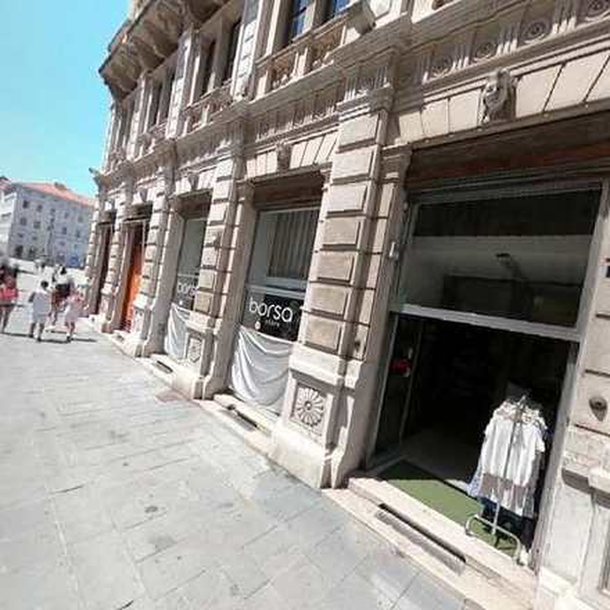
Here's a real, recorded frame from that pin loop — turn 3 of a claude-haiku-4.5 episode on eval task 40 (Trieste, Italy). The model called place_pin(45.6471, 13.7758) and got back exactly this and nothing more:
And the opening view of the same episode — the actual 90° street-level render the policy sees before any tool call, not a description of one:
The three methods, for real
The environment is one Python class, and what makes it a shippable environment rather than a private script is that both the trainer and a stranger with curl see the same two derived surfaces — an HTTP simulation API and an MCP tool surface — generated from one implementation:
class GeoGuesserEnvironment(MCPEnvironment):
    SUPPORTS_CONCURRENT_SESSIONS = True

    def reset(self, seed=None, episode_id=None, split=None, index=None, **kwargs) -> GeoGuesserObservation:
        """index picks one exact task, byte-identical on repeat -- what a GRPO
        group needs. seed picks tasks[seed % n_tasks]. Omitting both means
        genuinely random."""
        ...

    @property
    def state(self) -> GeoGuesserState:
        """Current internal state."""
        return self._state

    def _step_impl(self, action: Action, **kwargs) -> Observation:
        """Structured, non-MCP actions -- this is what MCPEnvironment.step()
        dispatches to for the HTTP /step route."""
        if isinstance(action, TypedAction):
            return self._apply(action)
        raise TypeError(f"Unsupported action type: {type(action).__name__}")
The part worth calling out structurally rather than as a code-reading exercise: /reset, /step, and /state — the simulation API a trainer drives — are registered by OpenEnv's server only when the process runs in simulation mode. A policy's only surface is /mcp, which carries tools and nothing else. So the property this whole design cares most about — that an agent under evaluation cannot reroll a task it dislikes — isn't a prompt instruction anyone has to trust. It's a route that doesn't exist in the deployment a policy actually talks to. That's a genuinely good piece of environment design, and it generalizes past GeoGuessr: whatever invariant matters most in your environment, ask whether it can be made structural instead of requested.
Determinism is the other half of what a GRPO group needs — eight rollouts of reset(split="eval", index=7) have to return byte-identical observations, or the group's "advantage" is measuring rendering noise instead of policy behaviour. Three things make that hold here: panorama bytes come from local disk instead of an expiring signed URL, reprojection is pure numpy with integer sampling, and the initial heading is pinned to the panorama's own compass_angle. OpenEnv makes reset(split, index) addressable; making it byte-identical is the environment author's job, not the framework's.
The reward: two curves, and a cliff that ate a third of the data
This is the article's most technically interesting design decision, and the one most worth checking arithmetic on rather than taking as narrated. Two reward curves exist in this project, on purpose, at more than 10× apart on the same guess.
The environment's own curve — what the leaderboard reports, what a human player would recognise:
where is distance in km and is accumulated action cost (0.01 per look/map, 0.02 per pin, 0.05 per move). What the trainer actually optimises:
Two changes: a second, five-times-slower decay scale, and a cost that multiplies instead of subtracting. Both look like knob-turning. Both change what's learnable, and the article's own numbers say by how much — I recomputed every one of the following from the two formulas above rather than trusting the stated conclusion:
Drag to 3,324 km and then to 18,723 km: the dashed game curve reads 0.0000 at both — a 5.6× difference in how wrong the guess was, and zero difference in what it scores. The solid trainer curve never floors: it keeps a second, 5,000 km decay scale alive under the first one, so a GRPO group of eight rollouts that all land on the wrong continent still has a gradient instead of eight identical zeros.
The single exponential is worth almost nothing across the exact range a weak model lives in. exp(-d/1492.7) peaks at 0.018 at 6,000 km and decays from there, so the entire 6,000–20,000 km range — where roughly a third of an untrained 4B's guesses land — carries no usable gradient. The 5,000 km scale is worth 0.150 at that same near edge, almost exactly the figure the article states.
Subtracting cost, then flooring at zero, collapses the ordering of bad guesses. I confirmed the exact mechanism directly from env/server/scoring.py's own docstring, which states the same number the article does: replaying 200 episodes through the game curve floors 77 of them at exactly 0.0, no variance between them — a 3,324 km miss and an 18,723 km miss score identically, and a GRPO group built from either has zero advantage. Solving the cliff in closed form, : at the board's cheapest reference arm (sonnet-5, mean cost 0.047) the cliff sits at 4,564 km — the article's "~4,500 km for a cheap episode." At the untrained 4B's own mean cost (0.108) it's 3,322 km — matching "~3,300 km at the average cost of these models" almost to the metre. (Averaging cost across all nine untouched reference arms instead gives 0.0998 and a cliff at 3,440 km — close, but the untrained 4B's own cost is the better match, which suggests that's the arm "average cost of these models" actually means.) Multiplying by a positive factor can never produce that collapse, which is the entire justification for the trainer's second formula.
De-risking: three checks, no GPU
Before spending money, the article runs three cheap checks, and the framing is worth keeping regardless of what environment you're building: a broken reward, a wrong turn budget, and a model that genuinely can't do the task all produce the same flat line at zero, and you cannot tell them apart from a loss curve after the fact.
Prove the environment can take the load, before the run. MAX_CONCURRENT_ENVS defaults to 4; four training ranks plus generation needs 8; and duplicate_space copies a Space's files but not its environment variables, so a duplicated Space silently keeps the default. A run against one of those dies an hour in with CAPACITY_REACHED: 4/4 sessions active. The check is six lines:
from geoguesser_env.client import GeoGuesserEnv
envs = [GeoGuesserEnv(base_url="https://<your-space>.hf.space") for _ in range(8)]
for e in envs:
    e.reset()
print("8/8 concurrent sessions OK")
Simulate the rollout with no gradient. Everything except the backward pass runs on a laptop against any served copy of the model. This is exactly how the article caught the bug that would have wasted a full run silently: the environment counted down its own budget of 24 turns, while the trainer's tool-calling loop stopped rollouts at 12. The model paced itself against the number in the tool result (24), was cut off at the trainer's real limit (12) before ever calling guess, and every reward came back exactly 0.0 — indistinguishable from a model that simply cannot learn the task. The fix is one regex stripping the environment's own countdown from what the model sees, so there is exactly one turn budget in play, ever.
Overfit two to four tasks before the real run. If reward doesn't climb toward the ceiling on a handful of tasks seen a hundred times, the model can't represent the task, the reward is broken, or the plumbing is broken — and any of those is much cheaper to learn for a few dollars than at hour nine of a real run. The metric to watch is frac_reward_zero_std, not reward itself: GRPO's advantage comes from spread within a group, so if most groups have zero spread, no amount of training fixes it, and the raw reward curve won't tell you that's what's happening.
Training run 1
model      Qwen/Qwen3.5-4B, LoRA r=16, alpha=32, dropout 0.05, on q/k/v/o_proj
hardware   4xA100 80GB, DDP under torchrun
steps      1000, at 1 task per step
rollouts   NUM_GENERATIONS=8, ACCUM=2 -> 8 episodes per optimizer step
episodes   8,000 total, touching 1,000 of 3,452 training tasks (29%)
optimiser  LR 3e-5, temperature 1.0, beta=0 (no KL anchor), scale_rewards="group"
cost       ~$102 training + ~$25 evals, 10.2 hours wall clock
hf jobs uv run \
--flavor a100-large --timeout 12h --image huggingface/trl --secrets HF_TOKEN \
-v hf://buckets/<you>/geoguesser-runs:/outputs \
-e OUTPUT_ROOT=/outputs -e MODEL=Qwen/Qwen3.5-4B \
-e ENV_URL=https://<your-space>.hf.space \
-e MAX_STEPS=250 -e SAVE_STEPS=25 -e MAX_COMPLETION=6144 \
grpo_geoguesser.pyThat's real, from train/README.md — and the article is upfront that the useful part of this run ends at step 250, which I'll come back to under the ablation.
The memorisation arithmetic checks out. 1,000 steps at 1 task/step touches at most 1,000 distinct training tasks (no repeats within a shuffled pass): 1,000 / 3,452 = 28.97%, which the article rounds to "29% of the split." Each touched task gets exactly one 8-rollout group, never repeated, and the 200-task eval split shares no sequence with training and sits at least 1 km from any training task — the contamination check above holds this exactly, not approximately. Memorisation isn't a live hypothesis here; the arithmetic rules it out before you even look at held-out accuracy.
The memory trap arithmetic checks out too, with a small honest wrinkle. The article's warning: max_completion_length sizes a logits tensor at length × vocab × 4 bytes, allocated regardless of what the model actually emits — at 12,288 tokens that's stated as reserving 11.4 GiB per step, against a longest real output of 2,114 tokens. Recomputing with the article's own stated vocabulary (248,064): 12,288 × 248,064 × 4 = 12,192,841,728 bytes = 11.355 GiB — rounds cleanly to "11.4 GiB." I checked that vocabulary figure three ways and none of them is exactly 248,064: Qwen/Qwen3.5-4B's own config.json lists text_config.vocab_size as 248,320; the shipped tokenizer's highest token id plus one is 248,077; the training script's own comment says "248064." None of the three differ from each other by more than 0.1%, and — this is the part that actually matters — recomputing the GiB figure with any of the three still lands at 11.35–11.37 GiB, all rounding to the same "about 11.4 GiB" the article states. A real, small, checkable imprecision in exactly which number is "the vocabulary," with zero effect on the conclusion it's used to support.
The two published adapters really are different weights, not a duplicate upload. Both geoguesser-qwen3.5-4b-grpo (run 1) and -v3 (run 3) list identical adapter_config.json hyperparameters — r: 16, lora_alpha: 32, lora_dropout: 0.05, target modules q_proj/k_proj/v_proj/o_proj (listed in a different order in each file, same set) — and both adapter_model.safetensors are exactly 12,592,424 bytes, which is simply what a fixed-rank LoRA over four fixed projections on the same base model weighs, regardless of what got learned. The Hub's file metadata gives each one a different sha256 (05d2438c... for run 1, a4d35f27... for v3) and a different repo commit sha — same architecture, same size, genuinely different trained weights, confirmed the way this site checks that kind of claim: by hash, not by file size.
What it actually learned
Fit over the nine reference dots only, r = -0.7500. The models that deliberate longest score worst, and it holds without either of the two arms anyone trained. Toggle in the untrained base and the fit softens to -0.720 — still strongly negative, just not quite as clean once a tenth point with 6.7 turns and 2.1 pins joins in.
The turns-vs-score correlation reproduces, to four decimal places, over the exact rows I can name. I computed Pearson's r on board.json's own numbers, over the nine arms tagged "reference" — every off-the-shelf model on the board that was never trained (claude-sonnet-5, gpt-5.4-mini, claude-haiku-4.5, Qwen3.5-122B-A10B, Qwen3.5-9B, Qwen3.5-35B-A3B, Qwen3.5-27B, Qwen3.5-397B-A17B, gpt-5.4-nano) — excluding both the untrained base and the trained checkpoint:
r(turns_per_episode, mean_of_4_score)  over 9 reference arms  =  -0.7501   (article: -0.75)
r(zero_scoring_share, mean_of_4_score) over 9 reference arms  =  -0.9649   (article: -0.96)
The article doesn't say which nine rows the number is over, which is exactly the kind of gap that makes a correlation unverifiable rather than wrong — so: those nine, above, excluding the arm that scored 0.4825 (the untrained base) and the one that scored 0.6445 (the trained checkpoint). Folding the untrained base back in moves r to -0.723 — still strongly negative, just measurably softer once a tenth point sitting at 6.7 turns and a 29.5% zero-scoring rate joins the fit.
The behavioural table is the headline, and it holds together internally. Every number below is the article's own, checked for self-consistency rather than independently re-run (I didn't retrain anything):
| checkpoint | score | turns | looks | tokens out | scored zero | median error |
|---|---|---|---|---|---|---|
| base | 0.4825 | 6.7 | 2.2 | 1062 | 29.5% | 1226 km |
| step 100 | 0.5600 | 2.6 | 0.6 | 186 | 18.5% | 964 km |
| step 200 | 0.6393 | 1.1 | 0.0 | 46 | 1.9% | 675 km |
| step 1000 | 0.6445 | 1.1 | 0.0 | 66 | 0.5% | 662 km |
Turns fall 6.7 → 1.1, looks go to zero, output tokens drop by an order of magnitude — and accuracy improves at the same time. That combination is the whole finding: the model didn't get lazier and worse, it got faster and better. Median error nearly halves; the share of episodes scoring exactly zero — which the article is careful to clarify is not "ran out of turns," since non-submission is nearly absent from this sweep, but guesses that landed past the reward's cliff (~3,300–4,500 km out) — falls from 29.5% to 0.5%.
I checked the reward-hacking ruled-out list, and the arithmetic behind it holds. A model that stops using its tools and scores better is the textbook shape of a reward hack, so the article spent a day looking for one: pin-loop leakage (ruled out — place_pin returns only what's at the coordinate, confirmed above), task-identity leakage (hide_task_identity=True strips task_index/task_id/sequence_id/attribution from every per-turn observation — I read this directly in _metadata() in geoguesser_environment.py, and the docstring there is specific about why: the Mapillary contributor username alone determines the country for 74% of training tasks, so leaving attribution in would let a policy score without reading the image at all), and memorisation (already checked above: 1,000 of 3,452 tasks touched, one group each, never repeated, scored against an eval split proven disjoint by full haversine check). None of it held up. What's left is that the largest available win on this reward was simply not being catastrophically wrong, and the fastest route there was committing to a first instinct instead of reasoning itself onto another continent.
The caveat the article volunteers is worth repeating, not burying. The 1.1-turn figure is measured under an eval protocol — JSON actions in text, only the current image visible — that the checkpoint never trained under (native tool calls, the full image history kept in context). Every arm on the board is measured the same protocol-consistent way, so the comparison is fair; the absolute number is protocol-dependent. The behaviour — glancing once, then committing — is real. "1.1 turns," specifically, is a property of how you choose to measure it, and the article says so itself rather than letting a clean number stand in for a messier truth.
The finished board
All eleven arms, same 200 held-out tasks, mean-of-4, 800 episodes per arm:
| model | mean-of-4 | median error |
|---|---|---|
| claude-sonnet-5 | 0.6952 | 324 km |
| run 1, step 1000 (Qwen3.5-4B + LoRA) | 0.6445 | 662 km |
| gpt-5.4-mini | 0.5732 | 753 km |
| claude-haiku-4.5 | 0.5374 | 939 km |
| Qwen3.5-122B-A10B | 0.5338 | 767 km |
| Qwen3.5-4B, untrained | 0.4825 | 1226 km |
| Qwen3.5-9B | 0.4776 | 1203 km |
| Qwen3.5-35B-A3B | 0.4483 | 1485 km |
| Qwen3.5-27B | 0.4478 | 1289 km |
| Qwen3.5-397B-A17B | 0.4466 | 1420 km |
| gpt-5.4-nano | 0.3748 | 2541 km |
The paired improvement over the untrained base, per-task, is +0.1620. I found the exact figure — including the confidence interval — sitting in the repo's own results/summaries/run1-full.txt, generated by eval/geoeval.py's report command, and it matches the article's headline number to four decimal places: delta +0.1620 +/- 0.0137, 95% CI [+0.1352, +0.1888], better on 169/200 tasks. That file is the actual regeneration artifact behind the prose, not a transcription of it. Reading the CI code directly — se = statistics.stdev(diffs) / math.sqrt(len(diffs)), 95% CI = mean ± 1.96·se — a paired normal approximation over 200 tasks, the stated ±0.0137 half-width backs out to an implied per-task standard deviation of the paired difference of 0.0989 (se = ci/1.96, stdev = se·√200). For a metric averaging 4 passes of a 0-to-1 score per task, a paired-difference spread of ~0.1 is exactly the kind of number you'd expect — not a red flag, and now you can check it yourself the same way.
The ablation: three runs, one confound resolved
Run 1 worked. The article ran two more, changing as little as possible each time, to find out why:
| run 1 | run 2 · 4B | run 3 | |
|---|---|---|---|
scale_rewards | group | none (Dr.GRPO) | group |
beta (KL anchor) | 0 | 0.02 | 0 |
| tasks per step | 1 | 2 | 2 |
| action cost scale | 1.0 | 0.2 | 0.2 |
| steps | 1000 | 300 | 300 |
| paired gain | +0.1620 | +0.0326 | +0.0717 |
| 95% CI | ±0.0137 | ±0.0090 | ±0.0105 |
Run 2 turned off advantage amplification and added a KL anchor, and kept 21% of run 1's gain (0.0326/0.1620). Run 3 reverted just those two knobs back, keeping run 2's other changes, and recovered 44% (0.0717/0.1620) — both fractions recompute exactly from the table's own numbers.
The comparison isn't step-matched, and the article's own progression table is what defuses it. Run 1 trained for 1,000 steps; runs 2 and 3 for 300. Read carelessly, "run 2 gained a fifth as much" could just mean "run 2 trained for 30% as long." But the same article's own checkpoint progression (in the section above) already shows step 200 at 0.6393 and step 500 at 0.6350 — run 1 had plateaued before step 300, the point where runs 2 and 3 stop. So the confound is real, and it doesn't bite: whatever run 1 gained by step 300, it had already gained almost all of by step 200, well inside the window runs 2 and 3 also trained in. Joining those two facts — the confound exists, and the plateau makes it not matter — is the kind of check this site exists to do, rather than either dismissing the ablation or treating the mismatch as fatal.
Run 1 vs run 3 still changes two knobs at once, not one: tasks-per-step (1→2) and action cost scale (1.0→0.2) both moved. The article names this itself and proposes the next experiment — change only the cost scale on top of run 3's config — rather than overclaiming isolation it doesn't have. Credit where it's due: that's the honest way to report an ablation you know is incomplete.
Every run carries its own frozen base arm, and the article preaches exactly this discipline elsewhere in the piece ("put a frozen base arm in every sweep... the same untrained model scored between 0.465 and 0.500 across our sweeps, a drift wider than most of the differences we wanted to claim"). The three Qwen3.5-4B base scores across the three runs — 0.4825 (run 1), 0.4768 (run 2), 0.4809 (run 3) — all sit inside that self-reported 0.465–0.500 drift band. That's the point made concrete: the same untrained model, measured three separate times across three separate sweep runs, and the spread between those three measurements is nearly as wide as some of the deltas the sweeps are trying to detect. (The run 2 · 2B arm's base of 0.4197 is a different, smaller model — it doesn't belong in that band and isn't claimed to.)
- task
- image-text-to-text
- library
- peft
- license
- apache-2.0
- safetensors
- 1 shard
- largest file
- 20.0 MB
- files
- 9
- downloads
- 13
- likes
- 0
repo last modified 2026-09-09
The advantage-amplification mechanism, from first principles
This is the most technically interesting claim in the piece: the instability in run 1 — the one that looked like a bug and drew two recommendations to kill the run — was the actual source of the learning signal.
GRPO computes an advantage for each rollout in a group by subtracting the group's mean reward and, when scale_rewards="group", dividing by the group's standard deviation:
The intent is sensible on its face: normalise so a group with naturally noisy rewards doesn't dominate the gradient over a group with naturally tight ones. The failure mode is what a "group" actually spans. At NUM_GENERATIONS=8 with one task per optimizer step (run 1's ACCUM=2 at per_device_batch=1, effectively one distinct task per step), the group's standard deviation is the spread of eight rollouts of the same location. As the policy gets more confident on that location — which is exactly what training is supposed to do — that spread shrinks toward zero, the divisor shrinks with it, and the same reward gap gets pushed harder every step it survives. It's a runaway loop with no external limiter besides epsilon in the denominator.
Run 1’s group std is the spread of eight rollouts of the same task, and it collapses: 32% of its steps sit in the lowest bin, implying a multiplier past 60×, with a measured ceiling near 10,000× when a group agrees exactly. Add a second task per step (run 2) and the group std also has to span the gap between two different tasks’ rewards, which a converging policy cannot shrink to zero — its distribution sits entirely above run 1’s collapse zone. Run 3 keeps two tasks per step but turns scale_rewards back to "group": the amplification comes back, just rarer — about 7% of its steps, not 32%.
I recomputed the medians directly from runs-std.json's per-step series rather than reading them off a chart: run 1's median group standard deviation across its 1,000 steps is 0.0155 (article: "0.016"), implying a typical multiplier of 1/0.0155 ≈ 64.5× (article: "~60"). Run 2, at two tasks per optimizer step, has a median of 0.1926 (article: "0.19") and a multiplier of ≈5.2× (article: "~5"), and its peak gradient norm of 0.158 matches the article's "peak grad norm 0.16" closely. Run 1's own peak gradient norm hit 11.25, matching "peaked above 11." At two tasks per step, the group's standard deviation also has to span the gap between the two tasks' rewards — a gap that doesn't shrink just because the policy is confident on either one individually — so the runaway loop structurally can't engage the same way.
Gradient accumulation is the coupling nobody warns you about here: ACCUM (or equivalently tasks_per_step) doesn't just change effective batch size, it changes what a "group" is allowed to span, which changes whether scale_rewards="group"'s denominator can collapse. That's a genuinely non-obvious interaction between two hyperparameters that look unrelated on a config sheet.
I went one step further than either the article's two data points and pulled run 3's own distribution from the same file, since it's published data nobody asked about yet: run 3 keeps two tasks per step (like run 2) but restores scale_rewards="group" (like run 1). Its median std is 0.0776, multiplier ≈12.9× — a genuine third point between the other two, not just a label. The full histogram makes it visual rather than a single number: run 3 spends about 7% of its steps in the same near-collapsed regime run 1 spends 32% of its steps in, and the rest of the time behaves like run 2. Pooling a second task makes the collapse rare, not impossible — which is exactly what the mechanism above predicts, and which neither the chapter text nor the published chart states explicitly.
What suppressing the instability cost: run 2 was designed, on purpose, to remove exactly the dynamics that made run 1 look dangerous — the entropy collapse (0.73→0.41) and the grad-norm spike were real signals, and stopping the run at either point would have been the reasonable-sounding call. Both times it would have been wrong. Turning that instability off with scale_rewards="none" (Dr.GRPO) and a KL anchor cost four-fifths of the eventual gain. The amplification wasn't a symptom of something broken — for this reward, on this task, it was most of the mechanism doing the actual work.
Six measurement bugs, and why they're the most reusable part of this
Every one of these produced a plausible-looking number. Exactly one of them ever threw an exception.
| bug | looked like | actually was |
|---|---|---|
| Wrong base served | 2B checkpoints scoring 0.469–0.479 | vLLM accepted 2B LoRAs on a 4B base and served anyway — all four scores invalid |
| Dead tunnel | a checkpoint regressing to 0.4475 | 13% of requests got an HTML 404 recorded as an empty reply; the episode burned its turns and scored 0 |
| Two reward scales | run 2's deltas incomparable to run 1's | stored reward is the environment's curve; reported deltas are recomputed through the trainer's curve. Same guess: 0.0107 vs 0.135 |
| No base arm | deltas read across sweeps | the same frozen base scored 0.465–0.500 between sweeps — wider than most of the differences being claimed |
Comparing across k | run 1 appearing to tie sonnet-5 | baselines read at pass@1 gave Sonnet 0.6798; at pass@4, 0.6952 — single-pass sampling noise, not a real gap |
| Concurrent sweeps | k = 1.8 with PASSES=1 | two sweeps writing to one output directory at once — arithmetically impossible, and the only tell |
I want to give this real space because it generalises far past GeoGuessr, and the "exactly one exception" framing is the actual lesson: a scoring pipeline that fails loudly on a config error is doing you a favour a scoring pipeline that fails quietly into a plausible-looking table never does. k = 1.8 with PASSES=1 set in the config is the only one of the six that couldn't have shipped as a real result — every other row would have looked like a legitimate finding to anyone who didn't already suspect something was wrong.
What this site's sibling articles add
Two other pieces here cover the same OpenEnv + TRL stack from different angles, and this one is closest to being the missing middle case between them. Scaling agentic RL covers Prime Intellect's agentic-task catalog, where the reward is a hidden test — ground truth exists, full stop, and the entire design problem is packaging it uniformly across 23 tasksets. Five judges were worth one opinion covers Hugging Face's own watercolour-painting environment, where there's no ground truth at all — the reward is a judge's opinion, or a preference model frozen after 1.17M human comparisons. GeoGuessr sits between the two: a real, objective ground truth (a lat/lon coordinate, a haversine distance), but a reward curve around that ground truth that has to be hand-shaped — the second decay scale, the multiplicative cost — to stay learnable at all. Ground truth existing isn't the same as the reward being trivial to write; this article is the clearest published example I've seen of that specific gap.
What I couldn't fully verify
In the interest of the same honesty the source article shows: a few things I checked as far as the published data allows and no further.
The 77-of-200 game-curve floor. I independently confirmed the mechanism (the closed-form cliff computation above) and found the exact same "77 of 200" figure sitting in env/server/scoring.py's own docstring — but reproducing the count itself needs the 200 raw per-episode distances from whichever specific pass@1 sweep it describes, and those aren't in the JSON files this article's charts are built from. The claim is corroborated by the source code stating the identical number independently of the article's prose; I did not re-run the 200 episodes myself.
An internal inconsistency, for the record. The repo carries a second, more detailed internal writeup, LEARNINGS.md, alongside the published article. It agrees with the published chapters almost everywhere, including the exact +0.1620/+0.0326/+0.0717 figures — but it states run 1 "touches only 58% of the 3,452-task split," while both the published chapter and my own arithmetic above land on 29% (1,000/3,452). 1,000/1,724 ≈ 58.0% almost exactly, which points at a training pool roughly half today's size — plausibly a stale note surviving a later dataset expansion that the published chapter's figure was updated for and this internal doc wasn't. Flagging it because even a team this careful about publishing raw data left one number inconsistent between two of their own documents, which is itself a useful reminder.
Reproduction
Everything I checked above is checkable again, with real commands: the environment is a playable Space, the task splits are the two JSONL files I ran the haversine check against, both trained adapters are on the Hub with hashes you can diff, every training run sits in one Trackio dashboard, and the code ships REPRODUCE.md with the exact command for every configuration in this piece, including results/summaries/, the actual geoeval.py report output the paired-CI numbers above came from.
Built on Adithya S Kolavi's How to turn a game into an RL environment: the technical intuition (Hugging Face, September 8, 2026), with every figure and table above either the article's own reported number (stated as such) or independently recomputed by me from the dataset splits, the JSON files behind the article's own charts (board.json, baseline-sweep.json, runs-ablation.json, run1-curve.json, run1-progression.json, runs-std.json, eval-tasks.json), the two published adapters' Hub metadata, and the actual source in 03-geoguesser (the environment class, scoring.py, grpo_geoguesser.py, geoeval.py, and LEARNINGS.md). The contamination check (690,400 pairs), both correlations, the ablation confound analysis, the advantage-amplification histograms, the vocabulary/memory arithmetic, the country distribution, and the Mapillary documentation check are all mine, run against their raw data rather than read off their charts. I did not retrain or re-evaluate any checkpoint myself, and did not independently reproduce the 77-of-200 game-curve floor or the LEARNINGS.md discrepancy beyond what's stated above. The two photographs are real recorded frames from a claude-haiku-4.5 episode in the published environment (flattened, resized, and attributed to the Mapillary contributor per CC BY-SA 4.0); the three interactive figures are my own, built from the article's published JSON, not redraws of their charts.