2026-10-06 · 18 min · llm · mixture-of-experts · open-weights · long-context · hybrid-attention · pretraining · explainer

Aleph Alpha released Kolibri-1 on 3 October 2026 with a four-line pitch: 78B parameters, 3.46B active, up to 1M tokens of context, built in Europe, weights under Apache 2.0. Behind it sits a 189-page technical report and, a week earlier, a blog post on scaling pre-training whose author has since said the "30B MoE" in it "was in fact Kolibri Origin all along" — the internal predecessor.
Three of those four numbers are architecture, and architecture can be checked. I pulled config.json,
read the header of every one of the 32 safetensors shards with HTTP range requests (no weights downloaded),
and recounted the model. Then I read the report for how the 1M context is reached, the blog for how the
training was scaled, and the evaluation tables for what the model actually beats.
Every number below carries a label. Measured means I computed it from a file. Reported means it is Aleph Alpha's figure and I did not re-run it. Reasoned means it is my arithmetic on the other two.
- architecture
- Kolibri1ForCausalLM
- task
- text-generation
- library
- vllm
- license
- apache-2.0
- safetensors
- 32 shards
- largest file
- 3.16 GB
- files
- 40
- downloads
- 2.5K
- likes
- 645
- languages
- de, en
repo last modified 2026-10-03
The shape, in one paragraph
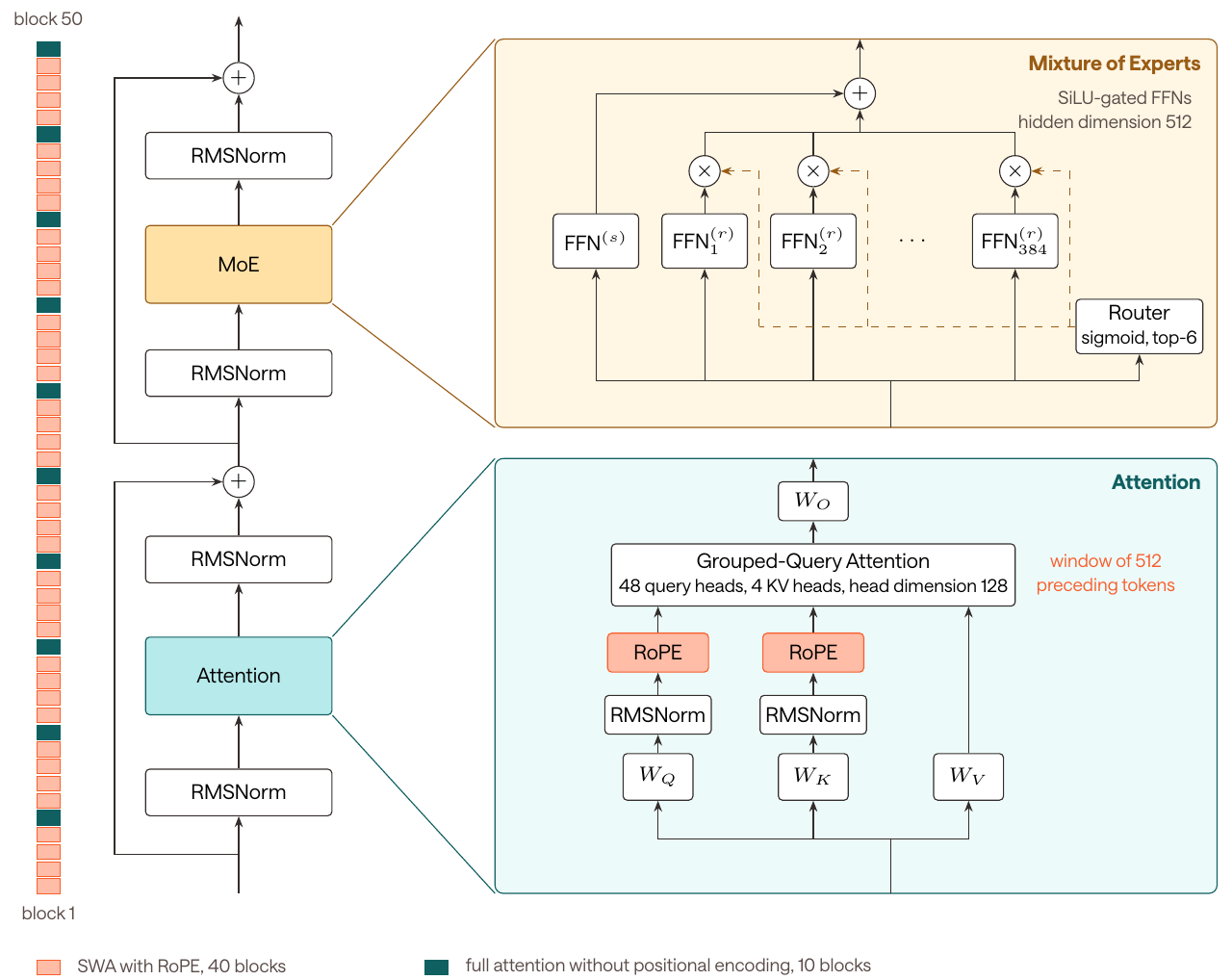
Kolibri is a decoder-only transformer with 50 blocks and a residual stream 2,560 wide. Each block has an
attention sublayer and a Mixture-of-Experts sublayer, each wrapped in a sandwich of RMSNorms (one before,
one after). Attention is grouped-query: 48 query heads share 4 key-value heads, head dimension 128. Every
fifth block is full causal attention with no positional encoding; the other 40 attend over a sliding
window of the 512 preceding tokens plus the current one, and only those 40 apply RoPE. The MoE layer holds
384 routed experts and 1 shared expert, each a SwiGLU FFN with hidden size 512; a sigmoid router
picks 6 routed experts per token. All of this is in config.json (measured) and the report's Figure 4.
Two config details are easy to miss. sliding_window is 513, not 512: the window counts the current
token, which matches the card's "512 preceding tokens plus the current token". And norm_topk_prob is
false: the six selected sigmoid scores weight the expert outputs as they are, without being rescaled to
sum to one (measured; the report says the same in its Equation 4).
Counting the parameters myself
The checkpoint is FP8 (float8_e4m3fn in 128x128 blocks, with an FP32 inverse scale per block), so the
shard sizes are not parameter counts. The headers are. Summing every tensor's shape, skipping the
weight_scale_inv tensors, gives 78,103,074,560 parameters (measured). That is exactly the card's
figure. The bytes add up too: 77,398,016,000 FP8 values, 705,058,560 BF16 values (embeddings, LM head,
norms, routers) and 4,724,000 FP32 scales come to 78,827,029,120 bytes, which is the total_size in
model.safetensors.index.json (measured).
Per block, from the shapes:
| Piece | Shape per block | Parameters per block |
|---|---|---|
| Attention (q, k, v, o + q/k norms) | 2560→6144, 2560→512 twice, 6144→2560 | 34,078,976 |
| One expert (gate, up, down) | 2560→512, 2560→512, 512→2560 | 3,932,160 |
| 384 routed experts | 384 x one expert | 1,509,949,440 |
| Shared expert | one expert | 3,932,160 |
| Router (weights + balancing bias) | 384 x 2560, plus 384 | 983,424 |
Add 50 blocks, a 128,000 x 2,560 input embedding, an untied LM head of the same size, and the norms, and you are back at 78.1B (measured).
Active parameters are what one token touches: attention, the shared expert, 6 of the 384 routed experts, the router, the norms and the LM head. The report excludes the input embedding, because it is a row lookup, not a matrix multiply. On that convention I get 3,457,570,560 (measured). The card says 3,457,573,120. The gap is 2,560 parameters, one vector of the model width; my guess is that their counter includes one norm vector differently, but I cannot see their counter, so that is unverified. Either way, 3.46B and 4.4% of the total (reasoned: 3,457,570,560 / 78,103,074,560 = 4.43%) both hold.
The widget recomputes every bar from the config fields. Three things fall out of it (all reasoned from the measured counts):
- 96.7% of the model is routed experts (75.5B of 78.1B), and a token uses 6/384 of them. That is the whole trade: a large store you must hold in memory, a small slice you multiply.
- Attention is 49.3% of the active parameters (1.70B of 3.46B). The routed experts a token actually runs are only 34.1% (1.18B). At this sparsity, the "small" part of the model, attention, does about half the matmul work per token. Moving top-k from 6 to 12 raises the active count to 4.64B, not to double.
- 2,560 x 512 experts are narrow. Each is 3.9M parameters. Kolibri's report tested this against a finer layout (512 experts, 12 active, width 2048) and a coarser one (256 experts of hidden size 1024, 6 active) at about 80B total, and the shipped shape had the lowest loss: 1.847 against 1.848 and 1.860 (reported, Appendix B.5.1). That is a small margin on one 327.6B-token proxy run.
For a broader treatment of why routed experts work at all, see the MoE architecture explainer and MoE from scratch.
Two layers that do not use their experts
The report contains a candid finding that the launch posts did not mention. Kolibri dropped the two leading dense layers its predecessor used, because a 327.6B-token ablation showed slightly lower loss without them (1.847 vs 1.850, reported, Table 5). In the full 20T-token run, though, the balancing bias ended up overriding the router in layers 0 and 1 almost completely: their top-K intervention rate reached 98.5%, near the 1 − 6/384 of a uniform choice. Randomising or silencing those two layers' routed experts changed held-out loss by an amount indistinguishable from zero (reported, Appendix B.6, Figures 54 and 55). An attempt to densify them during SFT gave no clear gain, so they shipped as they are.
That is 2 x 384 x 3,932,160 = 3.02B parameters, about 3.9% of the checkpoint, that the model does not rely on (reasoned). They still cost memory. The report says resolving it "remains future work". I find this more useful than another benchmark row: it shows a balancing method that looks healthy on the usual metrics (dead-expert fraction, router entropy) while silently randomising routing in the first layers.
Balancing: exact quantiles, not a histogram
Expert load is balanced by Exact Quantile Balancing (EQB), which follows the quantile-bias idea used in Kimi K3: each expert gets a bias that shifts the routing cutoff so that every expert receives its share of tokens over the global batch. The bias changes which experts are selected but not the weights the outputs are mixed with. The difference is in how the global quantile is computed across ranks: Kimi sums a 1,000-bin histogram per expert; EQB finds the exact BF16 quantile with a two-pass radix select over 256-bin histograms, which costs two all-reduces of 256 x 384 int32 counts per layer per step, independent of batch size (reported, Section 2.1.5). A second term, Load-Error Injection, pushes each microbatch toward balance through the score gradients (λ = 1e-5, τ = 1, reported). Over pre-training the global MaxVio averaged 0.31 across layers; layers 0 and 1 averaged 2.39 (reported).
How a 256k model reaches 1M
The 1M claim is the most interesting part of the design, and it comes from one decision about where positions live.
A full-attention layer with RoPE has a problem past its training length: it meets rotation angles for distances it has never seen, which is why long-context extensions usually rescale RoPE (YaRN and friends; see the RoPE explainer). Kolibri sidesteps it twice:
- The 40 window blocks have RoPE, but never see a distance over 512. Their attention mask stops at the window, so at token 1,000,000 a window block sees exactly the same relative positions it saw at token 600 in training.
- The 10 full blocks have no positional encoding at all (NoPE). They see every earlier token, but there are no angles to extrapolate. Order reaches them only through what the window blocks have already written into the residual stream.
So nothing in the network is asked to handle a position it was not trained on. The card's wording is
careful: trained at 262,144 tokens, "in principle" extendable to arbitrary lengths without position
scaling, and validated up to 1,048,576 (reported). In practice you must opt in: the shipped
config.json says max_position_embeddings: 262144 (measured), and serving 1M needs
--max-model-len 1048576 plus an --hf-overrides for that field (reported, from the card).
The report's own justification is an ablation at its small proxy scale: removing RoPE from the full-attention blocks "improved long-context performance" in early experiments, and a window of 512 beat 128 by 6.7 points at 256k at the 30.6B proxy scale, at a cost of 0.2 points on pre-training benchmarks (reported, Section 2.1.3). Qwen3.8-Flash-Next and Ling-3.0-flash reach the same 1M target with a different tool, linear attention, which keeps a fixed-size state instead of a fixed-size window; see Ling-3.0-flash and Qwen3.8 Flash Next.
What it costs in memory
The window also makes the KV cache simple to compute. Per block and per cached token, K and V take 2 x 4 heads x 128 = 1,024 values. A full block caches every token; a window block never caches more than 513.
With the FP8 KV cache the model was evaluated with (all reasoned from the config):
| Context | Kolibri (10 full + 40 window) | Same model, all 50 full |
|---|---|---|
| 4k | 63 MB | 210 MB |
| 256k | 2.71 GB | 13.4 GB |
| 1M | 10.8 GB | 53.7 GB |
The 40 window blocks always hold 21 MB between them, so past a few thousand tokens the cache is the 10 full blocks and the saving approaches 5x. The weights are 78.8 GB on disk (measured), so one B200 (192 GB) has room, before activations and fragmentation, for about 10 one-million-token sequences or 41 at the 256k trained length (reasoned). The report's own throughput analysis agrees on the mechanism: at long context "most of this long-context traffic comes from the 10 full-attention layers, while the 40 sliding-window layers read a fixed window and contribute negligibly" (reported, Section 2.1.4).
For the general GQA and KV-cache arithmetic, see the attention and KV cache explainer.
Does it actually work at 1M?
On RULER, the Kolibri base model scores 86.9 at 4k and 63.2 at 1M (reported). At 1M that is ahead of Nemotron 3 Nano Base (58.5) and Qwen3.5 35B-A3B Base (57.5, served with static YaRN), which is the case the design is built for. But at 4k Kolibri is second-lowest of the eight models in that table, above only Gemma 4 26B-A4B Base (84.7); Qwen3.5 Base scores 96.3 (reported). The curve is flat because it starts lower, not because it stays high. On HELMET it rises from 79.1 at 8k to 82.4 at 128k, behind Gemma 4 26B-A4B Base at every length (reported).
How the training was scaled
Kolibri pre-trained for 20T tokens at a 16,384-token context, then mid-trained on 3.44T at 65,536, then extended on 201B at 262,144 (reported). Pre-training ran on 768 B200s (96 nodes of 8) for 21 days, 392k GPU-hours, with the parallel layout EP 8, FSDP 16, DP 6: experts split across the 8 GPUs in a node over NVLink, dense weights sharded over 128 GPUs, six such replicas (reported, card and Section 2.1.6). The optimiser is Muon (spectral convention) on attention and expert matrices, AdamW or Adam on the rest; see the Muon article for the update.
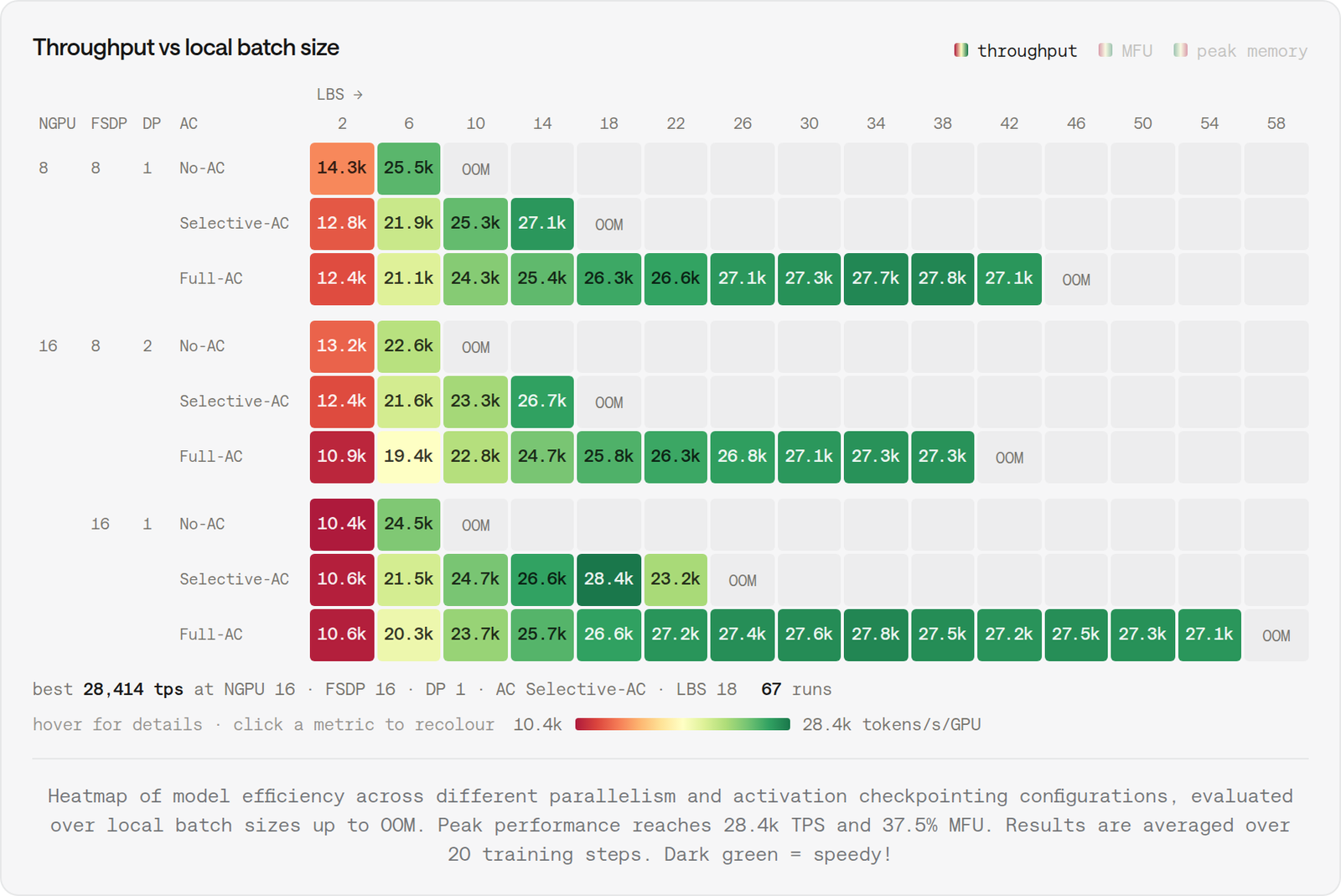
That run is easier to follow after the blog, which documents the method on the smaller model. The blog takes a 30B-A3B MoE from 16 to 512 B200s at a 4,096-token sequence and tunes three knobs: the sharding split between FSDP and DP, activation checkpointing (none, selective, full) and the local batch size. Its method is hierarchical. Sweep everything on 16 GPUs, where runs are cheap; keep only the regions that win; then scale FSDP until communication stops hiding behind compute; then scale DP, whose all-reduce is paid only on the last gradient-accumulation step (reported).
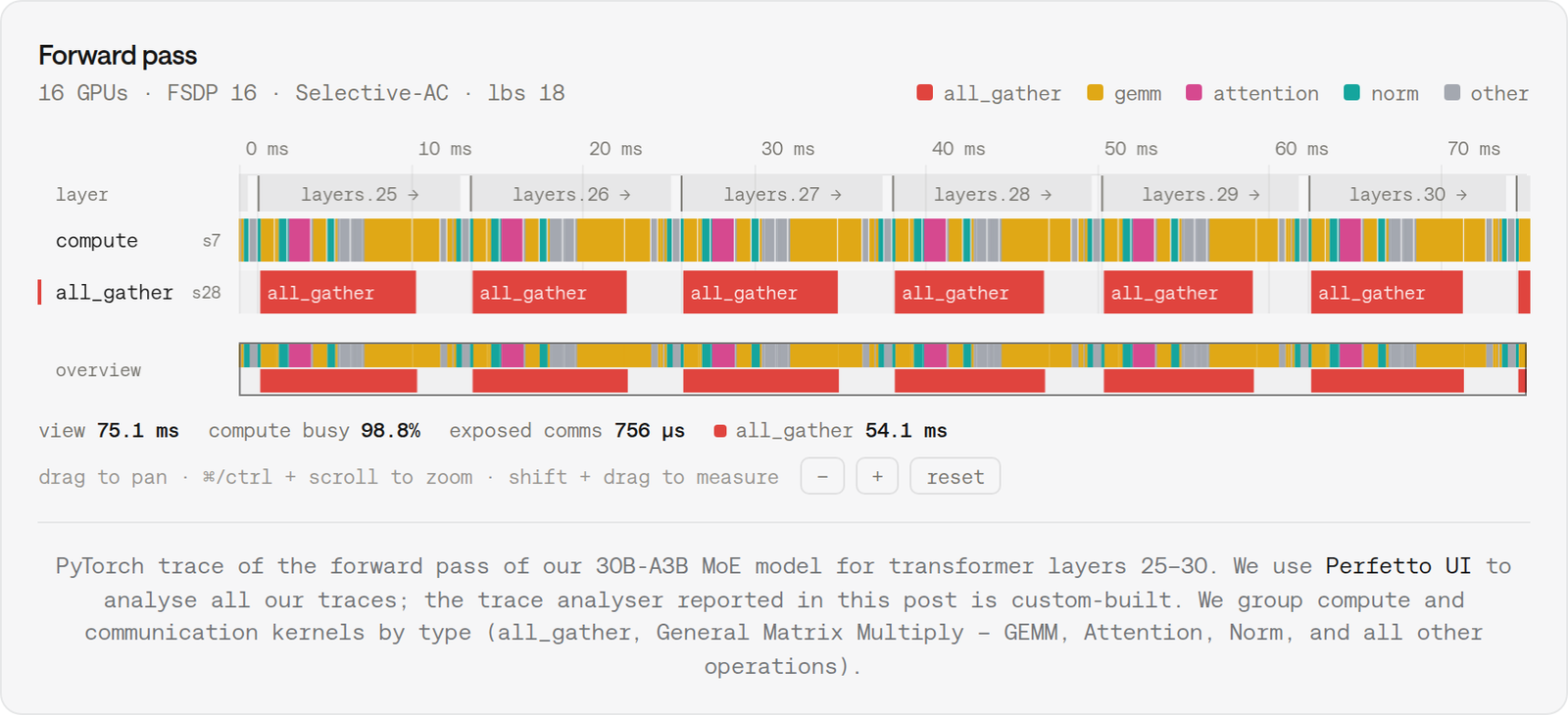
Profiling the winner showed the forward pass compute-bound: weight all-gathers for the next layer finish under the current layer's compute.
The blog's best configuration per scale (reported):
| GPUs | FSDP / DP | Tokens/s/GPU | MFU (BF16 peak) | HBM used |
|---|---|---|---|---|
| 16 | 16 / 1 | 28.4k | 37.5% | 92% |
| 128 | 128 / 1 | 28.0k | 37.0% | 93% |
| 512 | 128 / 4 | 26.7k | 35.3% | 94% |
The 6% per-GPU loss from 16 to 512 GPUs checks out (reasoned: 26.7 / 28.4 = 0.94), and so does the blog's "20T tokens on 512 GPUs within 17 days" (reasoned: 20e12 / (26.7e3 x 512) s = 16.9 days). The Ai2 comparison is in the Olmo-core 3 article, which read this blog before anyone knew which model it was about.
Now line the blog up with the report. Kolibri Origin is listed as 30.6B total, 3.27B active, pre-trained on 7.5T tokens at a 4k context (reported, Part 2 and Table 2). A 4k context matches the blog's fixed 4,096-token sequences, which supports the "Origin all along" claim; I have only the author's word that it is the same run's configuration (reported, unverified).
The more interesting line is one the blog wrote about itself: expert parallelism was out of scope, but "if our model were larger or sparser, we would likely need EP." Kolibri is both: 2.5x the total parameters and 4.4% active against Origin's 10.7% (reported). And its layout is the one the blog anticipated: EP 8 inside the node, FSDP and DP across nodes, with DeepEP for the dispatch (reported, Section 2.1.6 and Appendix B.7).
What the report does not give is an MFU for the Kolibri run. It gives throughput: per-run medians of about 16.5k tokens/s/GPU at 16k sequences, flat over 264,750 steps after an early dip (reported, Figure 56). The card's total of 20T tokens in 392k GPU-hours averages to 14.2k tokens/s/GPU including restarts and checkpoints (reasoned). Counting only parameter matmuls, 6 x 3.46B FLOPs per token at 16.5k tokens/s is about 342 TFLOP/s per GPU (reasoned), before attention. I will not turn that into an MFU, because the denominator depends on which B200 peak you pick, and the blog itself warns against comparing MFU across setups. The card's total of 6.4e23 FLOPs is also reported, not reproduced: 6 x 3.46B x 23.64T tokens is 4.9e23 (reasoned), so their count is about 30% higher, presumably attention at long sequences. I cannot verify their accounting.
The benchmarks, read honestly
Aleph Alpha's headline result is a Pareto plot: average score against decoded bytes per second per GPU, every model in its fastest configuration on eight B200s.
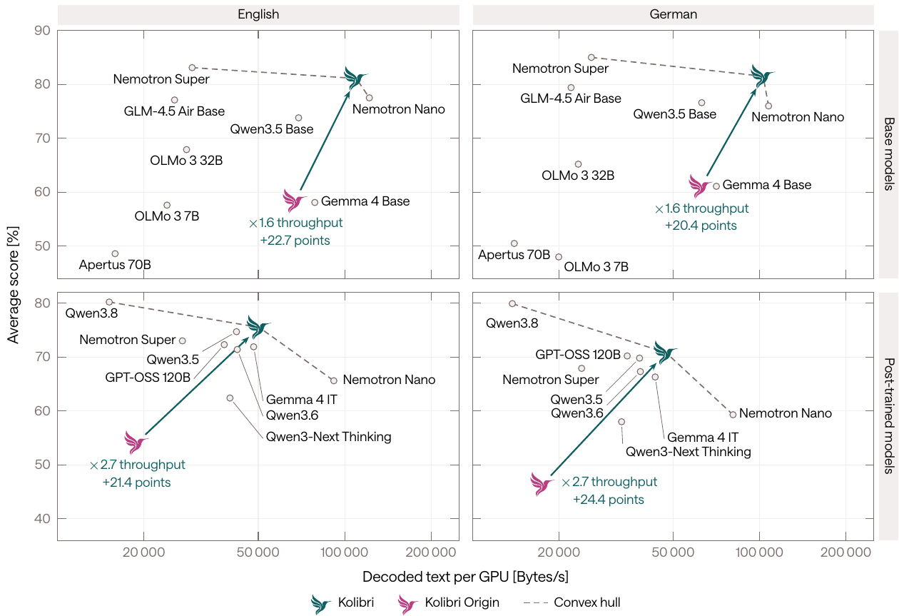
The plot measures bytes, not tokens, which is the fair choice for a model whose tokenizer packs German tighter (4.90 bytes per token on German web text, against 4.35 for GPT-5's, reported). Being on the hull means no evaluated model is both faster and better. It does not mean best: post-trained Qwen3.8 27B, a dense model, averages 80.2 English against Kolibri's 75.5 (reported) at lower throughput.
All scores below are Aleph Alpha's own runs, with their eval framework, Kolibri at reasoning effort
high (reported). I did not re-run any of them.
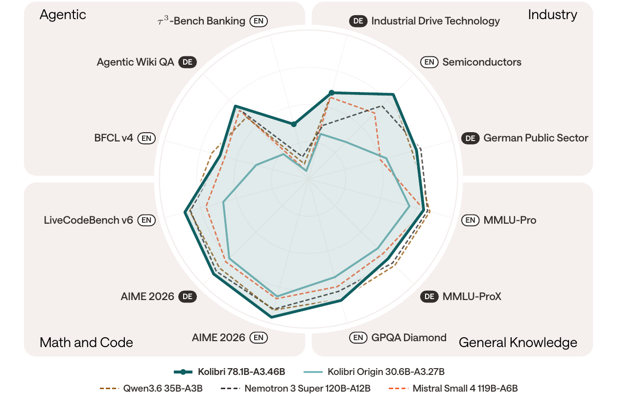
One launch thread claims Kolibri "beats Qwen 3.5 35B, Nemotron 3 Super, and Mistral Small 4" in math, science and code. The figure that thread shows is the report's Figure 2, which compares Qwen3.6 35B-A3B, not 3.5. Checking both against the tables:
| Benchmark | Kolibri | Qwen3.5 35B-A3B | Qwen3.6 35B-A3B | Nemotron 3 Super | Mistral Small 4 |
|---|---|---|---|---|---|
| AIME 2026 (EN) | 96.0 | 92.1 | 91.0 | 90.4 | 83.1 |
| GPQA Diamond (EN) | 84.3 | 83.8 | 83.4 | 78.0 | 74.7 |
| GPQA Diamond (DE) | 81.3 | 84.2 | 80.6 | 76.6 | 72.9 |
| LiveCodeBench v6 | 85.9 | 77.8 | 82.5 | 82.0 | 71.2 |
| SWE-Bench Verified | 66.4 | 71.6 | 73.8 | 60.2 | 60.8 |
| MMLU-Pro (EN) | 80.0 | 84.6 | 84.3 | 82.7 | 80.4 |
(reported, model card post-training table)
The claim holds for competition math and LiveCodeBench, by a wide margin. On GPQA English it holds by half a point, inside what I would call noise. It fails on German GPQA against Qwen3.5, on SWE-Bench Verified against both Qwens, and on MMLU-Pro. "Math, science and code" is two of three, with code split by benchmark.
The weak spots are where you would expect a small active count to show: stored knowledge and hallucination. AA-Omniscience accuracy is 14.8, below all ten external MoE models in the table, and RGB fact-checking is 34.0 against 74.0 for Qwen3.5 (reported). The flip side is trained abstention: Kolibri's AA-Omniscience non-hallucination rate is 44.0, second among the MoE models only to Qwen3.6's 56.7 (reported). It knows less and says so more often. For RAG over a company's own documents, which is the deployment the report describes, that is the right failure mode; the "Industry RAG" average is 89.7 English, the best MoE score (reported, on Aleph Alpha's own industry sets, which no one else has run).
German is the other half of the pitch. The German overall average is 70.8, best among the MoE models, with GPT-OSS 120B at 70.2 (reported). That gap is 0.6 points.
What I would take from it
Kolibri is a careful, well-documented model rather than a frontier one. The parts that are new are small and specific: positions only where distances are short, a window just large enough to hold up at 256k, exact global quantiles for balancing, and a tokenizer trained for German compounds. Together they buy a cheap long context: a 10.8 GB KV cache at 1M tokens in FP8, against 53.7 GB if every layer were full.
What it costs is memory you must hold for experts that mostly sleep: 78.8 GB of weights to run 3.46B parameters per token, 3.02B of them in two layers the model does not need. The card's minimum is two H100s or one B200. If your bottleneck is GPU memory rather than decode throughput, a dense model in the same quality band will fit where Kolibri does not.
And the training story is a nice case of a blog post that turned out to be a preview: the 16-to-512 GPU method was worked out on Kolibri Origin, and the expert parallelism it deferred is exactly what the 78B model needed.