Qwen's RL formulation: token-level RL is a first-order approximation to the reward you want
mdjsonmcp2026-07-24 · 11 min · reinforcement-learning · mixture-of-experts · post-training
Why read this
Nichelast 15%Why token-level RL is the first-order part of the sequence objective, and when to use R2 or R3 Routing Replay for MoE, from Qwen's stabilization paper.
- Widely used
- A lasting reference
- A new technique
Training & RLNeeds datacenter GPUsResearch paper
How this was scored
- Is it new?
- 2 of 3: A real new idea, method or capability
- Can I trust it?
- 0 of 3: Restates claims
- Can I run it?
- 0 of 3: Closed, nothing to run
- Will I understand it?
- 2 of 3: Mechanism from first principles with figures
- Can I act on it?
- 2 of 3: A concrete recipe, numbers or comparison
- Will it last?
- 2 of 3: A reference for a year or more
- Does it affect many?
- 2 of 3: A widely used model, tool or lab release
- Only here?
- 1 of 3: Some original analysis
Score 47 of 100, ranked 495 of 577 rated articles. Each question is answered 0–3 by hand, and a 3 is rare. How articles are scored
RL for reasoning models rests on a mismatch nobody had really justified. The reward is assigned to a whole response — you sample a full chain of thought, check the final answer, and hand back one scalar. But the optimizer — REINFORCE, GRPO, and the rest — works one token at a time. We reward the sequence and update the tokens, and we mostly just trust that closing the loop this way improves the thing we scored.
The Qwen team's Stabilizing Reinforcement Learning with LLMs (Zheng et al., arXiv:2512.01374) takes that trust and makes it a theorem with fine print. Their claim: the token-level objective is a first-order approximation to the true sequence-level reward — exact in the limit, and valid only when two specific gaps are small. The nice part is what falls out of it. Importance-sampling correction, clipping, and Routing Replay for Mixture-of-Experts models — a grab-bag of stabilization tricks that each arrived with its own justification — turn out to be the same move: keep the approximation valid. One lens, and the whole toolbox lines up behind it.
The objective you can't optimize
Write the thing we actually want to maximize — expected reward over responses the current policy would generate:
There's an immediate wrinkle: we don't sample from the policy we're training. Responses come out of a fast inference engine (vLLM, SGLang) running policy , while gradients are taken in a training engine (Megatron, FSDP) holding . The standard fix is an importance-sampling reweight onto the rollout policy :
This is correct and completely impractical. A sequence likelihood is a product of hundreds or thousands of per-token probabilities, so the ratio swings across an enormous dynamic range with brutal variance. Its gradient is technically right and numerically hopeless. Nobody trains on it directly.
The surrogate everyone actually uses
So instead we optimize the token-level objective — sum the per-token IS ratios instead of multiplying them:
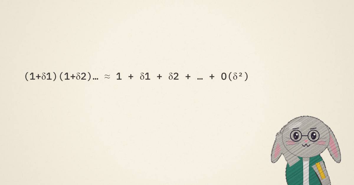
Its gradient is just REINFORCE with a per-token IS weight — stable, cheap, the workhorse of every modern RL post-training run. The paper's key move is to show why it's allowed to stand in for the sequence objective. Write each token ratio as with small. Then the true sequence ratio is a product, and a product of near-ones is, to first order, one plus the sum:
Drop the terms and the gradient of the intractable sequence objective becomes exactly the gradient of the token surrogate. That's the whole theorem: the token-level objective is the linear part of the sequence objective. They agree when the per-token ratios hug 1, and they part ways as those ratios drift — because the neglected second-order cross terms are precisely what the linear surrogate throws away. Drive the two gap sources and watch the true product pull away from the surrogate:
The intuition to keep: the surrogate isn't wrong, it's truncated. As long as the policy you're optimizing stays close to the policy that generated the data, the truncation is negligible and improving the cheap objective improves the real reward. Let them separate and the surrogate starts optimizing something that isn't the reward anymore — which, in practice, is exactly what a training collapse looks like.
Two gaps, and the tricks that close them
"Keep close to " sounds abstract until you factor the token ratio into its two honest sources:
- Training–inference discrepancy is numerical. The same weights produce slightly different probabilities in the training and inference engines — different kernels, and inference deliberately disables batch-invariant kernels for throughput, so even one engine isn't self-consistent. This is the gap between and .
- Policy staleness is procedural. To use more compute per rollout, we split a big batch of responses into mini-batches and take several gradient steps, so later mini-batches are optimized by a that has already drifted from the that generated them. Asynchronous frameworks make it worse.
Now the stabilization toolbox reads as one idea — shrink these two gaps so the first-order approximation holds:
- The IS weight itself is not an optional variance trick; it is the first-order term. Drop the training–inference correction and you're no longer approximating the sequence objective at all.
- Clipping (the PPO move) stops gradients on tokens whose ratio has run too far, directly capping policy staleness.
- Routing Replay, for MoE models, closes both — and it needs its own section, because MoE breaks the story in a way dense models don't.
Why MoE breaks it, and how Routing Replay repairs it
In a Mixture-of-Experts model, the probability of a token depends on which experts the router activated for it. That turns the token ratio into a comparison over possibly different active parameters: the inference engine routes the token to expert set , the training engine to , and when those sets disagree the ratio stops measuring "a small change in the policy" and starts measuring "two different subnetworks." The are no longer small, and the first-order approximation collapses. Routing is entangled with both gaps — the engines can route differently (discrepancy) and the router's choice can shift as weights update (staleness). Toggle the fix:
Routing Replay (Zheng et al., 2025; Ma et al., 2025) pins the routed experts during optimization so the token is scored over one fixed subnetwork — the model is optimized like a dense one, and the ratio means what it should again. The paper formalizes two flavors, differing only in whose routing you replay:
| replays | closes | first mini-batch | |
|---|---|---|---|
| R2 — Vanilla Routing Replay | the training engine's rollout experts | policy staleness | target policy unaltered |
| R3 — Rollout Routing Replay | the inference engine's experts | discrepancy and staleness | target policy altered |
There's no free lunch here, and the paper is careful to say so. Fixing the experts restores the approximation but biases the target policy — you're now optimizing a model whose routing is frozen to a past choice, not the routing it would pick itself. R2 leaves the first mini-batch's target policy untouched; R3 alters it from step one but kills more of the discrepancy. Which bias is worth paying turns out to depend on how off-policy you run — a question only experiments can settle.
MiniRL: the smallest honest baseline
To test the formulation instead of a pile of confounded tricks, the authors strip RL down to MiniRL — REINFORCE with the token-level IS weight, group-normalized advantages (subtract the per-prompt mean reward), and PPO-style clipping. That's it. It's deliberately the minimal algorithm whose gradient stays faithful to the surrogate the theory justifies, which makes it the right probe: if the formulation is real, the things that preserve the approximation should be the things that stabilize MiniRL.
The setup is a genuine stress test. A 30B MoE (cold-started from Qwen3-30B-A3B-Base), FP8 inference against BF16 training — deliberately mismatched precisions to inflate the training–inference discrepancy — on 4,096 verifiable math problems, scored as average accuracy over 32 samples on HMMT25, AIME25, and AIME24. Hundreds of thousands of GPU hours, roughly 5–6 GPU-hours per gradient step. They track not just reward but two diagnostics: policy entropy and the training–inference KL divergence, since a collapse announces itself as a KL spike before the score falls.
What the experiments say
On-policy (one gradient update per batch), the ablation lands exactly where the theory predicts:
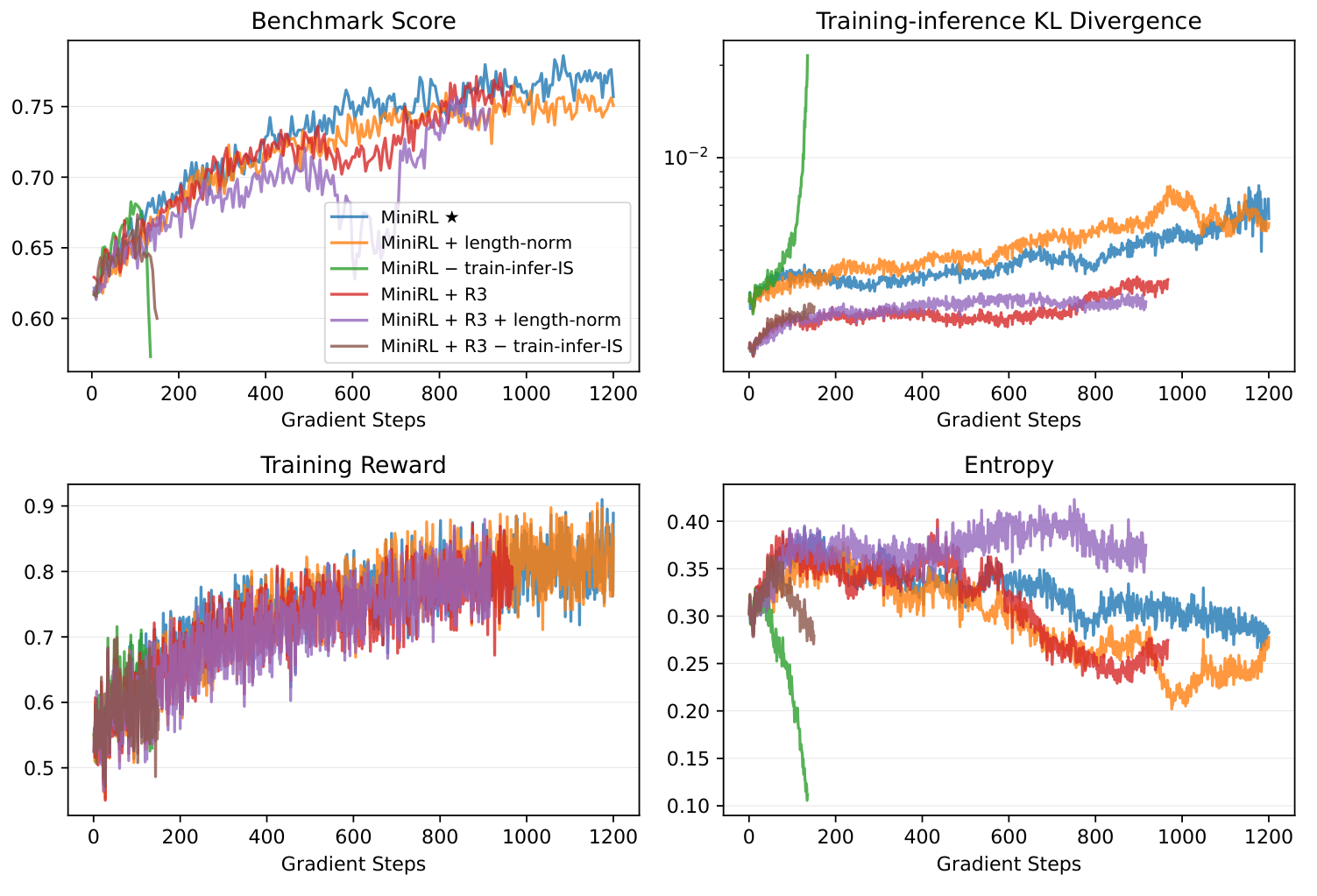
Three reads, each a prediction of the formulation:
- MiniRL wins. The plain first-order-faithful objective is the most stable and scores highest.
- Removing the training–inference IS correction collapses training almost immediately — the green curve nose-dives, entropy crashes, KL explodes. The IS weight was never optional; it's the approximation's load-bearing term.
- Length normalization is stable but worse. Dividing the objective by response length is common (GRPO and CISPO both do it), but it invalidates the first-order approximation — the gradient no longer lines up with the true sequence objective — and the benchmark score pays for it. Notably, Routing Replay does not help on-policy; with the gaps already small, its bias is all cost and no benefit.
Off-policy (split the batch into mini-batches for updates), staleness enters and the picture changes. Now clipping and Routing Replay both become necessary — drop either and training collapses early:
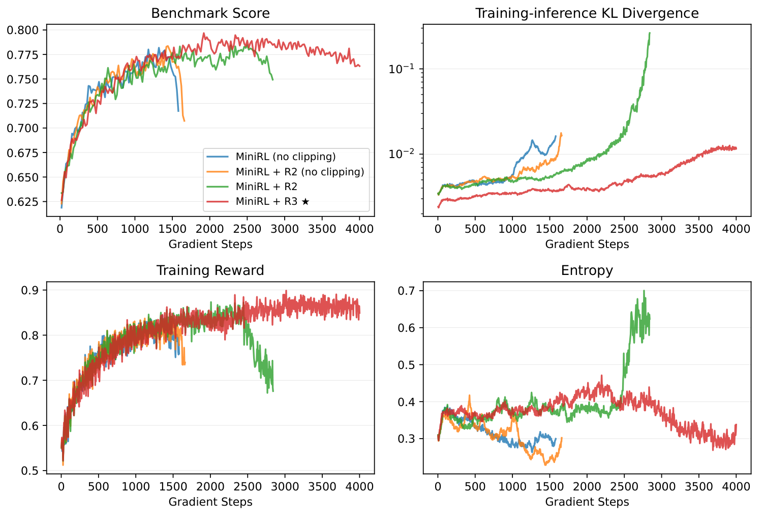
The nuance the paper draws out: at small off-policiness (), R2 beats R3 — R2's lighter bias wins when the approximation is only mildly stressed. At larger off-policiness (, ), R3 wins — R2 can't hold training together and R3's stronger discrepancy-killing earns its bias back. The recipe isn't "always use X"; it's "match the replay to how off-policy you're willing to run."
The result that reframes the field
The finding I keep coming back to isn't a trick — it's about what matters. Take one base model, cold-start it three different ways (distilling from Qwen3-Max-Thinking-Preview, DeepSeek-R1-0528, and gpt-oss-120b), then run the same stable recipe. They converge to the same place:
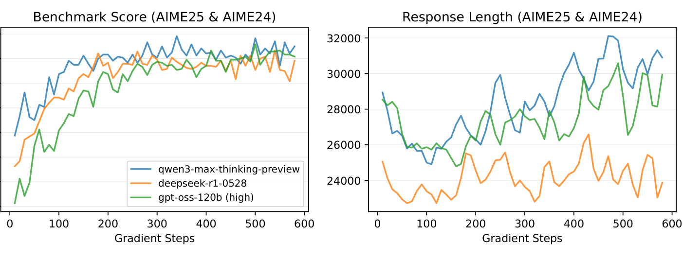
Once training is stable, how you started barely matters — prolonged RL washes out the cold-start differences and even on-policy and off-policy runs reach comparable peaks. The implication is pointed: the field spends enormous effort curating cold-start data, and this says that effort is mostly erased by enough stable RL. The lever that actually moves the ceiling is stability, not initialization.
The take
- One approximation, one toolbox. Token-level RL is the first-order truncation of the sequence objective. IS correction, clipping, and Routing Replay aren't three unrelated patches — they're three ways to keep the truncation valid by shrinking the training–inference discrepancy and policy staleness.
- The IS weight is structural, not cosmetic. It's the linear term itself; removing it doesn't add variance, it changes what you're optimizing, and training collapses on contact.
- MoE needs Routing Replay, and it's a real trade. Pinning experts restores the ratio but biases the target policy. Use R2 when you're near on-policy, R3 when you push off-policy — the paper's clearest practical recipe.
- Stability is the scaling lever. Different cold-starts, on-policy vs off-policy — once stable, they land in the same place. The honest limits: one task, one model family, a stress-test precision setup, and headline benchmark values read from curves rather than a table. The formulation is the durable part; the exact numbers are a single, if very large, data point.
Built on Stabilizing Reinforcement Learning with LLMs: Formulation and Practices (Zheng et al., Qwen Team, Alibaba). Routing Replay's two flavors trace to GSPO (R2) and Ma et al., 2025 (R3, arXiv:2510.11370). Figures are the paper's; the interactive diagrams are mine.