2026-09-19 · 18 min · explainer · webgpu · browser-ml · on-device-inference · architecture · llm
The question was whether a Jev-shaped model could run in the reader's own tab.
The argument for trying is in the CUA-S1 piece:
a per-option scalar scorer is an encoder plus a head whose output dimension is
one. No autoregression, no KV cache, no sampling loop. One forward pass per
option, a scalar out, a softmax over the scalars afterwards. That is the easiest
possible thing to put behind onnxruntime-web.
So I built it rather than argued about it. It is directly below, it downloads nothing until you click, and it prints the latency and the backend it got.
It works. The rest of this piece is what measuring it taught me, which is not what I expected going in, and includes one thing I could not measure at all.
- architecture
- GLiClassModel
- task
- text-classification
- library
- transformers
- license
- apache-2.0
- safetensors
- 1 shard
- largest file
- 606.3 MB
- files
- 11
- downloads
- 309
- likes
- 11
The only open System One model that ships an actual in-browser playground. Read its ONNX export rather than its README: the graph's output is logits[batch, 25] — the candidate capacity is welded into the exported tensor shape, not left as a loop bound.
repo last modified 2026-09-17
What the demo actually is
Three NLI cross-encoders, from the Hub, through
transformers.js 4.3.0 on ONNX
Runtime Web. An NLI cross-encoder is a per-option scalar scorer with a different
name on it: you hand it (context, hypothesis) pairs, it returns a small fixed
row of logits per pair — three for the MNLI checkpoints, two for the ModernBERT
one — and you keep exactly one column, the entailment logit, as that option's
score. BertForMultipleChoice has worked this way since 2019, and it is the
same one-scalar-per-option shape CUA-S1 trains from scratch.
// components/articles/jev-in-the-browser/browser-scorer.tsx
const inputs = await tokenizer(
  live.map(() => context),                          // the same context, N times
  { text_pair: live.map((o) => `This example is ${o}.`),
    padding: true, truncation: true, max_length: 256 },
)
const { logits } = await model(inputs)              // [N, 2 or 3]
const scalars = rows.map((r) => r[spec.entailIndex]) // one number per option
const probs = softmax(scalars)                       // softmax AFTER, over N
Nothing in that code knows how many options there are. live.length is a loop
bound, the option strings are data, and you can edit them in the widget and
watch the distribution move. That much of the premise holds completely.
Two engineering notes, because they are the whole reason it is safe to put on a
page. The library is imported inside the click handler —
await import("@huggingface/transformers") — so it is never statically
reachable from the server build, and a reader who scrolls past downloads zero
bytes. And the size is printed before the button, not after.
The bill, itemised
A per-option System One scorer in the browser costs a WASM runtime before it costs any weights, and that runtime is larger uncompressed than the smallest model in the ladder. Loading the default model in the widget on this page transferred 90.45 MiB across 18 requests, measured in the real page rather than read off a model card.
| fetched | kind | uncompressed MiB | transferred MiB |
|---|---|---|---|
| ort-wasm-simd-threaded.asyncify.wasm (jsDelivr) | runtime | 25.62 | 5.29 |
| transformers.js bundle | runtime | 1.28 | app chunk |
| nli-deberta-v3-xsmall — model_quantized.onnx (q8) | weights 70M | 83.2 | 83.2 |
| nli-deberta-v3-xsmall — tokenizer.json | weights 70M | 8.26 | 1.94 |
| mobilebert-uncased-mnli — model_quantized.onnx (q8) | weights 25M | 25.72 | — |
| mobilebert-uncased-mnli — tokenizer.json | weights 25M | 0.68 | — |
| ModernBERT-large-zeroshot-v2.0 — model_q4f16.onnx | weights 395M | 283.61 | — |
| ModernBERT-large-zeroshot-v2.0 — tokenizer.json | weights 395M | 3.42 | — |
| rlcd-modernbert-151m — model_fp16.onnx (303,785,047 B) | weights 151M | 289.71 | — |
| rlcd-modernbert-151m — model.onnx (606,323,181 B) | weights 151M | 578.24 | — |
| TOTAL for one click on the default model, in the real page | 18 requests | — | 90.45 |
The .onnx weights barely compress — they are already-quantised tensor data — while the WASM runtime and the tokenizer JSON compress by 4-5x. That is why the runtime looks frightening uncompressed and is tolerable in practice, and why the weights are the number that decides whether you ship this. The two rlcd-modernbert-151m rows are exact byte counts from the Hub for the only open System One model with a browser playground; it publishes no int8 or 4-bit export at all.
Two things in that table are worth saying out loud.
The runtime is not free and nobody counts it. Before a single weight
arrives, the page fetches ort-wasm-simd-threaded.asyncify.wasm — 26.9 MiB
of ONNX Runtime plus the transformers.js bundle. That is larger than the
smallest model I benchmarked. Every "we shipped a 25 MB model to the browser"
claim is really a 52 MiB claim unless the runtime was already cached from
somewhere else. It does compress — jsDelivr served that same file to this page
as 5.29 MiB on the wire, a 4.8× saving, which is the number in the
transferred column. The weights do not: .onnx files of quantised tensors
come back the same size they went in.
The open System One models do not ship a small export. The one model in this
whole story built for the browser,
heman10x/rlcd-modernbert-151m,
publishes exactly two ONNX files: model.onnx at 606,323,181 bytes and
model_fp16.onnx at 303,785,047 bytes. Both are on the Hub; I downloaded and
ran both. There is no int8 and no q4 export, which means the cheapest possible
first load of the only open System One model with a browser playground is
290 MiB of weights, before the 27 MiB of runtime. Compare that against the
same demo's own pitch — "runs locally in browsers via WebGPU/WASM" — and the
pitch is true and the number is the thing that decides whether you would.
The thing I could not measure
There is no GPU in the machine I write these on. /dev/dri does not exist.
Chrome still gives you WebGPU — it falls back to Dawn on SwiftShader, a software
Vulkan rasterizer — and the adapter says so plainly:
{ vendor: "google", architecture: "swiftshader", device: "", description: "" }
I ran the WebGPU path anyway, because "does the code path work" is a different question from "is it fast". The code path works: the session built in 6,653 ms and every forward pass completed. It is not a performance measurement of anything. Six consecutive two-row forward passes of a 25M-parameter MobileBERT took 11.3 s, 12.9 s, 11.9 s, 16.7 s, 21.1 s and 25.3 s. The same batch on the WASM backend, same tab, same minute, is a couple of hundred milliseconds.
So: I cannot tell you what Jev-in-the-browser costs on a real GPU, and I am not going to pretend a software rasterizer is a proxy for one. What I did instead is make the demo report your adapter and your latency. If you are reading this on a machine with a GPU, the number in that widget is the measurement this section is missing, and it is a better one than I could have produced here.
The latency, honestly
One disclosure before the numbers: this is a shared 4-vCPU VM that spent the session at a load average between 7 and 18, so the spread between runs is wide and the medians are contaminated. Under noisy neighbours the minimum over many runs is the least-corrupted statistic, so that is the column to read; the median is there to show you how bad the noise was.
One decision, N options, per-option scalar scoring, in a browser tab on a CPU with no GPU. Latency grows with the option count because each option carries its own copy of the context; read the min column, because the machine was contended.
| model | options | tokens | min ms | p50 ms | max ms |
|---|---|---|---|---|---|
| MobileBERT-MNLI 25M q8 | 2 | 96 | 178.41 | 484.04 | 871.73 |
| MobileBERT-MNLI 25M q8 | 5 | 255 | 207.61 | 351.61 | 923.5 |
| MobileBERT-MNLI 25M q8 | 16 | 816 | 280.71 | 934.52 | 1,567.83 |
| DeBERTa-v3-xsmall NLI 70M q8 | 2 | 88 | 72.76 | 128.29 | 214.07 |
| DeBERTa-v3-xsmall NLI 70M q8 | 5 | 230 | 159.7 | 172.1 | 265.67 |
| DeBERTa-v3-xsmall NLI 70M q8 | 16 | 752 | 437.09 | 472.83 | 675.88 |
| ModernBERT-large zeroshot 395M q4f16 | 2 | 92 | 1,210.48 | 1,261.82 | 1,433.13 |
| ModernBERT-large zeroshot 395M q4f16 | 5 | 240 | 2,520.41 | 2,724.27 | 4,382.09 |
| ModernBERT-large zeroshot 395M q4f16 | 16 | 784 | 11,425.96 | 17,654.46 | 32,560.92 |
| MobileBERT — 16 separate passes, not one batch | 16 | 816 | 609.66 | 638.31 | 700.27 |
| DeBERTa-v3-xsmall — 16 separate passes, not one batch | 16 | 752 | 711.29 | 795.35 | 1,816.69 |
| ModernBERT-large — 16 separate passes, not one batch | 16 | 784 | 30,761.9 | 38,161.63 | 54,082.25 |
These are local compute, not a network round trip. Jev's published p50 of 236-338 ms is an HTTPS request to someone else's datacentre and includes TLS, queueing and distance; comparing the two numbers directly is meaningless and is not what this table is for. The last two rows show the same 16-option decision run as 16 separate one-row forward passes instead of one padded batch of 16.
Latency grows with the option count. For the DeBERTa model it grows roughly with the token count — 88 → 230 → 752 tokens against 73 → 160 → 437 ms, so a 8.5× token increase buys a 6.0× time increase. For the 25M MobileBERT it grows far more slowly, because at that size the fixed cost of a call (tokenising in JS, marshalling tensors across the WASM boundary) is a large fraction of the total and the actual matrix multiplies are almost free.
The row that decided the design of the widget is the third model. A 4-bit ModernBERT-large — the same class as Laya's 395M backbone, which is the closest public stand-in for an open Jev — needed 11.4 seconds at best and 32.6 at worst for one sixteen-option decision on the WASM backend, and 30.8–54.1 s if you run the sixteen options as sixteen separate passes. That is not a slow widget, it is a frozen tab, which is why the 395M option in the demo is disabled unless your browser hands back a WebGPU adapter.
And here is the part that decides whether any of this is worth shipping. I ran the same ticket past all three models twice, with two plausible sixteen-option support taxonomies for the same job.
The same ticket, the same architecture, two plausible sixteen-option support taxonomies. The 25M model is wrong on both. The 70M model is right only when the correct option is spelled out, and by 5.7 points. The 395M model is right on both and knows it. This is the accuracy half of the ladder whose latency half is in the table above.
| model | MiB | terse list — top answer | p | explicit list — top answer | p |
|---|---|---|---|---|---|
| MobileBERT-MNLI 25M q8 | 26.4 | a complaint about support response time ✗ | 0.235 | a chargeback already filed with the bank ✗ | 0.251 |
| DeBERTa-v3-xsmall NLI 70M q8 | 91.5 | a question about pricing ✗ | 0.308 | a duplicate charge that needs refunding ✓ | 0.453 |
| ModernBERT-large zeroshot 395M q4f16 | 287 | a duplicate charge dispute ✓ | 0.659 | a duplicate charge that needs refunding ✓ | 0.952 |
N = 1 decision per cell. This is a demonstration of the failure mode, not an accuracy benchmark, and it is reported that way: nobody should conclude a ranking of these three models from six decisions. What it does establish is that at the sizes that fit comfortably in a browser, the answer depends on how the caller phrased the options — which is a property of the whole category, not of these checkpoints.
The 25M model is wrong both times. The 70M model — the fast one, the one I made the default — is wrong on the terse taxonomy and right on the explicit one by 5.7 points over "a question about pricing". Only the 395M model, the one that takes eleven seconds, is right both times, and the gap between its answer and its runner-up is 33 points on one list and 94 on the other.
So the ladder is not "small and fast versus big and slow". It is fast and wrong versus right and unusable, and the middle rung's correctness depends on how the caller happened to word the options. A confident wrong answer in 437 ms is worse than no answer, and that — not the download, not WebGPU — is the hardest thing about putting this category in a browser.
One caveat I want to be loud about: that is one decision per cell, six in total. It is a demonstration of a failure mode, not a benchmark, and nobody should rank these three checkpoints from it. What it does show is that the failure mode exists at the sizes that fit in a tab.
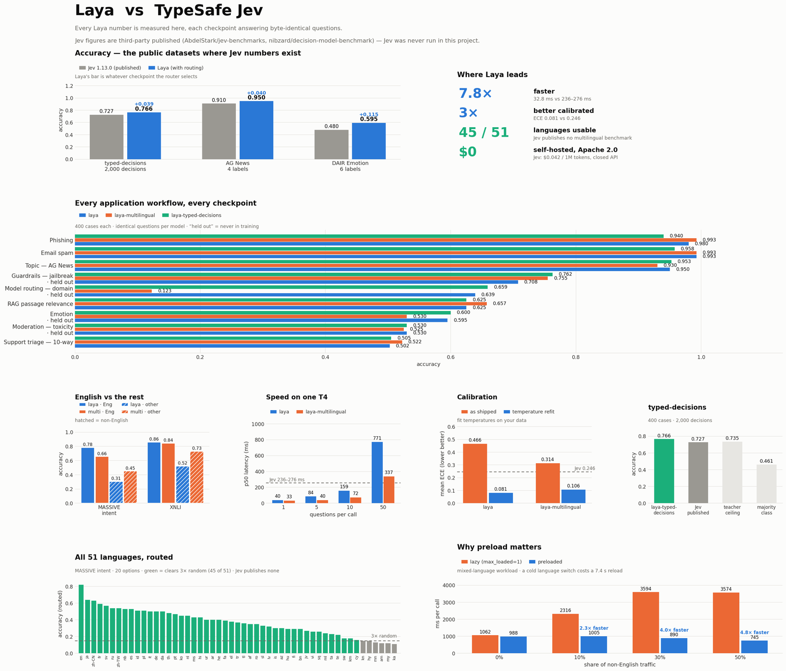
Now the comparison everybody wants, with the caveat that makes it legal. Jev's published round trip has been independently measured at 236–276 ms p50 by AbdelStark and nibzard, and at 338.6 ms by Paras Chopra. My 437 ms at sixteen options is in the same neighbourhood as those numbers and the two are not comparable: one is compute on a contended CPU with no GPU, the other is an HTTPS round trip to a datacentre that includes TLS, queueing and the speed of light. Strip the network from one side and the comparison evaporates. The only honest claim is the weak one — a 91 MiB int8 encoder on four contended CPU cores lands in the same order of magnitude as a hosted API call, which tells you the hosted figure is dominated by something other than the model's arithmetic, and tells you nothing about the model.
The confidence is a function of your option list
Having the thing running locally means you can poke it in ways an API bill discourages. Here is the experiment that came out of that, and it is the result I did not expect to find.
Start with the widget's five default options. The correct one scores 0.619. Now add a paraphrase of it — "a double charge that should be reversed" — and score again. Then another. Then a third.
Adding paraphrases of the right answer to the option list collapses the probability the model reports for it — from 0.619 to 0.215 — while the belief itself does not move. A 0.5 act/escalate threshold acts at five options and abstains at six, on identical evidence.
| paraphrases added | options | logit of original | p(original) | p(concept) | argmax |
|---|---|---|---|---|---|
| 0 | 5 | 2.293 | 0.619 | 0.619 | a duplicate charge that needs refunding |
| 1 | 6 | 2.12 | 0.482 | 0.589 | a duplicate charge that needs refunding |
| 2 | 7 | 2.031 | 0.265 | 0.762 | a payment taken twice that needs returning |
| 3 | 8 | 2.184 | 0.215 | 0.821 | a repeated charge awaiting a refund |
The logit of the original option should be exactly invariant — each option is encoded and scored in its own row, so nothing another option does can reach it. It drifts by at most 0.26 across these four runs because the padded batch width changes as options of different lengths join it, and DeBERTa-v3's disentangled attention is a function of the sequence length. That drift is two orders of magnitude too small to explain the probability collapse, which is entirely the softmax denominator growing.
The probability of the right answer falls from 0.619 to 0.215 while the model's belief in the concept rises from 0.619 to 0.821. Nothing about the evidence changed. Nothing the model thinks changed — the raw entailment logit of that option sits at 2.29, 2.12, 2.03, 2.18 across the four runs, drifting only because the padded batch width moves. What changed is the denominator.
This is not a bug in my code or in the checkpoint. It is arithmetic. Each option is encoded in its own row and scored in isolation, then the softmax is taken over the scalars, so the probability an option receives is a function of what else the caller happened to list. Put three phrasings of the same answer on the list and they share the mass between them; the concept's total goes up, every individual number goes down.
Now put a policy on top, which is the entire reason this category exists — act autonomously above 0.5, escalate below. That policy acts at five options and abstains at six, on identical evidence, because somebody added a synonym to a dropdown. The calibration you are relying on is calibrated against your option list, not against the world.
And the isolated shape cannot fix this, in the strong sense: an option's score is computed without any access to the other options, so no amount of training can teach it to notice that three of them mean the same thing. A model whose options share a sequence at least can learn to. Hold onto that, because the next two sections are the same trade seen from two other angles.
Where it actually gets interesting
Watch the option count in the widget. Every option you add costs a whole extra row, and every row carries its own copy of the entire context. That is not an inefficiency in my code; it is the isolation guarantee. TypeSafe's own description of Jev — "every level is evaluated separately. The model doesn't see a level's number or its neighbours" — is precisely a promise that no option ever shares a sequence with another option, and the only way to keep that promise is to encode the context again for each one.
rlcd-modernbert-151m build actually is, read from its own worker.js: all candidates are <<LABEL>> spans in one sequence. Right is the shape a browser wants. It is also the shape that cannot make the isolation guarantee.The alternative shape puts every option in one sequence as a marked span, encodes once, and reads N logits out. Price both, with one tokenizer, on identical content:
Xenova/nli-deberta-v3-xsmall), counted both ways. The isolated shape pays a fresh copy of the context for every option — 49 tokens a row here, so 784 at sixteen options. The shared-sequence shape pays the context once and then only each option’s own words: 126. That 6.2× is not an implementation detail to optimise away; it is what “the model doesn’t see a level’s neighbours” costs, stated in tokens.6.2× at sixteen options, and the gap widens with N because one curve is
linear in N × |context| and the other is linear in Σ|option|. That is the
cost of option isolation, stated in the one unit that does not depend on my
machine's load average, my backend, or my quantization.
And this is exactly where a browser hurts most. On a datacentre GPU, 784 tokens versus 126 is a rounding error against the fixed cost of a kernel launch. In a tab, on whatever laptop the reader has, it is the difference between a widget that feels instant and one that does not.
Both open System One models already made this trade
This is the part that changed my mind while writing.
Laya is the 421M ModernBERT-large
open System One, and its own architecture section says how it scores: "every
option is scored at its own [MASK] token, then softmaxed over that question's
options", with a "512 tokens per question (question + options + state)" budget
and "every question in a call is answered in one forward pass". That is the
right-hand column of the diagram above. All options, one sequence.
- task
- text-classification
- library
- transformers
- license
- apache-2.0
- safetensors
- 3 shards
- largest file
- 842.6 MB
- files
- 38
- downloads
- 0
- likes
- 499
Scores every option at its own [MASK] token inside a single 512-token sequence — the shared-sequence shape, not the isolated one. Its own latency table is measured on a Tesla T4, not a browser.
repo last modified 2026-09-19
rlcd-modernbert-151m is the same choice made a different way: it is GLiClass
over ModernBERT-base, and its browser worker builds the prompt by hand —
// webgpu-demo/worker.js, from Heman10x-NGU/Verdict-open-jev
const labelPrefix = candidates.map(c => `${promptContract.label_marker}${c.desc}`).join("");
const prompt = `${labelPrefix}${promptContract.sep_marker}${formattedText}`;
label_marker is <<LABEL>> and sep_marker is <<SEP>>, from the committed
prompt_contract.json. Every candidate is a span in one string, ahead of one
separator, ahead of the question and the context. One session.run, all
candidates.
So the two open models that actually ship an edge or browser story are both uni-encoders, and they are fast in a browser because they are. They bought that speed with the property the whole category is named for. The relational-choice result is the same trade seen from the other end: Jev scores 0 of 100 on questions where one option's content decides another, and it scores zero precisely because the options never meet. Laya scores 8. A 4-bit Qwen3-4B, which sees everything at once, scores 53.
You can have option isolation or you can have one forward pass. Nobody has shipped both.
The export welds N into the graph
One more thing, and it is the finding I would keep if I could keep only one.
The CUA-S1 piece closed on "N is a loop bound, not a weight." That is true of every one of these models in PyTorch. It stops being true when you export for the browser. Here is the graph metadata of the only open System One ONNX export I could find:
$ python3 -c "import onnxruntime as ort; s=ort.InferenceSession('model.onnx', providers=['CPUExecutionProvider']); \
  print([(i.name,i.shape) for i in s.get_inputs()]); print([(o.name,o.shape) for o in s.get_outputs()])"
[('input_ids', ['batch_size', 'sequence_length']), ('attention_mask', ['batch_size', 'sequence_length'])]
[('logits', ['batch_size', 25])]
batch_size is symbolic. sequence_length is symbolic. 25 is not. The
candidate capacity is a literal in the exported tensor shape, which matches
"max_capacity_logits": 25 in the repo's bundle_manifest.json and
"max_candidates": 25 in prompt_contract.json, and the demo's worker enforces
it with a thrown error. I ran the graph at 2, 5, 16 and 25 candidates and the
output was [1, 25] every time; the extra rows are sliced off in JavaScript
afterwards.
So in the browser the option set is no longer data. It is a shape, chosen at export time, and going past it is a re-export rather than a longer array. That is a small, concrete, checkable way in which the architecture that makes this category interesting does not survive the trip to the edge intact — and it is invisible from the model card, which advertises "25 candidate slots" as a feature rather than as an export constraint.
What I would actually ship
If I wanted a System One model in a production page tomorrow:
- Not the 421M or 395M class on a CPU. ModernBERT-large at 4 bits is 283 MiB of weights on top of 27 MiB of runtime, and 11–33 seconds per sixteen-option decision without a GPU. It is the only model here that answers correctly, and it is not shippable on the fallback path. Gate it on an adapter or leave it out.
- A ~91 MiB int8 cross-encoder is the fastest honest option if isolation matters to you — 437 ms at sixteen options on a CPU with no GPU — with the caveat that at that size it got one of my two sample decisions wrong, and the other one right by less than six points. Measure accuracy on your own decisions before you measure anything else.
- If isolation does not matter, use the uni-encoder and say so. Six times fewer tokens, one pass, and you can answer the relational questions the isolated shape cannot. Just do not then claim the property you traded away.
- Gate the download on a click, print the size first, and cache it. This is not a performance tip. A multi-hundred-megabyte fetch triggered by scrolling is a bug.
The answer to "can we run Jev in the browser" is yes, with an asterisk that is more interesting than the answer: the part of Jev that is hard to run in a browser is not the model, it is the guarantee.
What would change my mind
5 claims above, and what would falsify each
Option isolation costs ~6× the tokens of a shared-sequence packing at sixteen options.
Re-tokenise any real decision workload both ways with one tokenizer and count. The ratio is roughly
N × |context| / (|context| + Σ|option|), so it falls toward 1 when the context is short and the options are long. If your traffic is two-word contexts and paragraph-long options, the gap I measured collapses and my framing is wrong for your case.A real GPU does not rescue the isolated shape's scaling, it only shifts the constant.
I could not test this — no GPU here. Run the widget above on a machine with one and compare latency at 2 versus 16 options. If the ratio is near 1.0 because sixteen rows fill the GPU no better than two did, then on GPUs the isolation tax is free and this article's central point applies only to CPUs and phones.
The 25 in rlcd-modernbert-151m's ONNX output is an export constraint, not a model property.
Load the safetensors checkpoint in PyTorch and run 26 candidates. If it errors the same way, the capacity is in the weights and I have described the export wrongly. If it returns 26 logits, the constraint arrived with the export and my reading holds.
The WASM latencies here are contaminated by machine load, not representative of the method.
This one I am asserting against myself. The load average sat between 7 and 18 on four vCPUs and the min-to-max spread reached 4.9×. Run the same models on a quiet machine — the widget does exactly this — and if the minima I report are more than ~30% off a quiet box's median, treat every absolute millisecond in this article as indicative only. The token counts and byte counts are unaffected either way.
In a per-option scorer the reported probability is a function of the caller's option list, not only of the evidence.
Duplicate an option in the widget above and score again — it is two clicks. If the winning probability does not fall by roughly the amount the duplicate takes, my reading of the softmax is wrong. The stronger version: do it against the hosted Jev API and check whether the same collapse appears. If Jev's probabilities are stable under paraphrase, it is doing something after the per-option softmax that nobody has described, and that would be the most interesting undocumented thing about it.
Everything measured here was measured on 19 September 2026 on a 4-vCPU Linux VM with 15 GiB RAM and no GPU, in headless Chromium 141 driven by Playwright, with transformers.js 4.3.0 over ONNX Runtime Web 1.31.0-dev. Model weights: Xenova/mobilebert-uncased-mnli, Xenova/nli-deberta-v3-xsmall, onnx-community/ModernBERT-large-zeroshot-v2.0-ONNX, and heman10x/rlcd-modernbert-151m with its source at Heman10x-NGU/Verdict-open-jev, cloned and read rather than summarised. Byte counts are response body sizes recorded by the browser, not figures from a model card — including the 90.45 MiB total, which is what the widget on this page actually transferred when a script drove it end to end. Token counts come from the tokenizers themselves. The ONNX graph shapes come from onnxruntime reading the downloaded file, and the redundancy experiment ran through the same code path the widget uses. Laya's architecture and latency quotations are from its own model card. Companion pieces: A System One model in 706,048 parameters for the two families, Jev scores zero for what isolation costs in accuracy, and Tiny browser models for the other end of the size range.