Fly wiring, scrambled wiring, same score

oruk.ai published a piece called "We taught a fruit fly to hear human emotion" (Nathan Roll, September 6, 2026). The headline is exactly as clickable as it sounds: they took 499 real neurons from a fruit fly's wiring diagram, copied the connections into software, ran human voice recordings through it, and trained a readout to predict the emotion labels people gave those recordings. There is a genuinely gorgeous interactive 3D reconstruction of the actual traced neurons. I want to talk about all of that — but I want to lead with the part of the post most people will scroll past, because it's the most important thing on the page:

That is the authors, in their own methods section, reporting the control that undoes their own headline — and putting it in the main body of the post, not buried in an appendix. That is rare, and it deserves real credit before anything else. So here is the honest version of this piece: what's actually going on is reservoir computing, a well-established technique where a fixed, untrained recurrent network does the heavy lifting and only a small linear readout gets trained on top of it. The reservoir happens to be shaped like a fly brain. That shape, per the authors' own control, doesn't seem to matter. What does the actual work — and what the post explains unusually well — is one scalar: the network's spectral radius.

expand

499 neurons, one weight formula

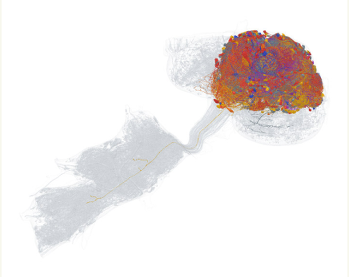
The connectome comes from MaleCNS v1.0, the male fruit-fly central-brain reconstruction from FlyEM at HHMI Janelia with Cambridge, the MRC Laboratory of Molecular Biology, and Google Research. The authors took the 512 strongest eligible central-brain intrinsic neurons — traced cells with modeled transmitter signs and at least five contacts per edge — and kept the largest strongly connected component: every neuron can reach every other neuron through some directed path. That component has 499 neurons, wired by 15,865 connections backed by 867,344 synaptic contacts.

expand

Turning a wiring diagram into weights needs a few choices the anatomy doesn't supply on its own, and the post is candid about that:

"A connection in the model gets stronger when the reconstruction contains more synaptic contacts. We also assign positive or negative signs using neurotransmitter annotations. These are engineering choices: a wiring diagram does not supply every receptor, time constant or physiological detail needed to simulate the original cells."

Concretely: each weight starts as sign × log(1 + contact_count), then the whole matrix gets one global rescaling. Signs come from neurotransmitter identity — acetylcholine positive, GABA and glutamate negative — which the post flags plainly as "model assumptions," not measurements. None of this is wrong to do; it's the standard way anyone turns a connectome into a simulatable network. But it's worth sitting with how much is decided by the modeler rather than read off the fly: the time constants, the nonlinearity, the input pathway, and — as it turns out — the global rescaling are all synthetic. What the anatomy actually contributes is a sparsity pattern: which of the 499×499 possible connections exist at all, and roughly how strong each one is relative to its neighbors. Everything else is added.

This is reservoir computing

Here's the part that matters most. The network's dynamics are:

with $W$ globally rescaled so its spectral radius — the magnitude of its largest eigenvalue — hits a target of 0.9. That's a leaky-integrator echo state network (ESN): a fixed recurrent reservoir driven by an input, with only a small readout ever trained on top. Feed a signal in, and "each neuron combines that input with the previous activity of its neighbors and retains part of its own previous state" — the post's own description, and a fair one. This exact idea — drive a fixed biological connectome as a reservoir and read out its activity — isn't new: Suárez et al. built conn2res specifically to study connectomes this way, and Costi et al. have already used a fruit-fly connectome for time-series prediction. oruk's contribution is applying the same recipe to listener judgments of speech — a new application, not a new method.

Why does spectral radius get top billing over the wiring itself? Because it controls whether the network has the echo state property: does it eventually forget its own starting state and settle into a trajectory that depends only on recent input? Below a spectral radius of roughly 1, yes — any two starting states, driven by the same input, converge. Push it past 1 and they don't; the network keeps chewing on its own history instead of just tracking the input, and a linear readout fit to one run's activity has no reason to generalize to another. 0.9 sits deliberately just under that edge — enough recurrent memory to be useful, not so much that the state stops being a reliable function of the input. Drag the sliders below and watch it happen in a small (24-unit, not the fly's 499) fixed random reservoir — same input, two different starting states:

That threshold is a property of the scalar $\rho$, not of which pattern of connections you rescale to hit it. Which is exactly why a scrambled network — same degree sequence, same signs, same weight values, rescaled to the same 0.9 — behaves almost identically to the fly's own wiring. The connectome supplies a sparsity pattern; the spectral radius supplies the physics; and the physics is what a ridge readout actually gets to see.

The input is random too, and the readout is small

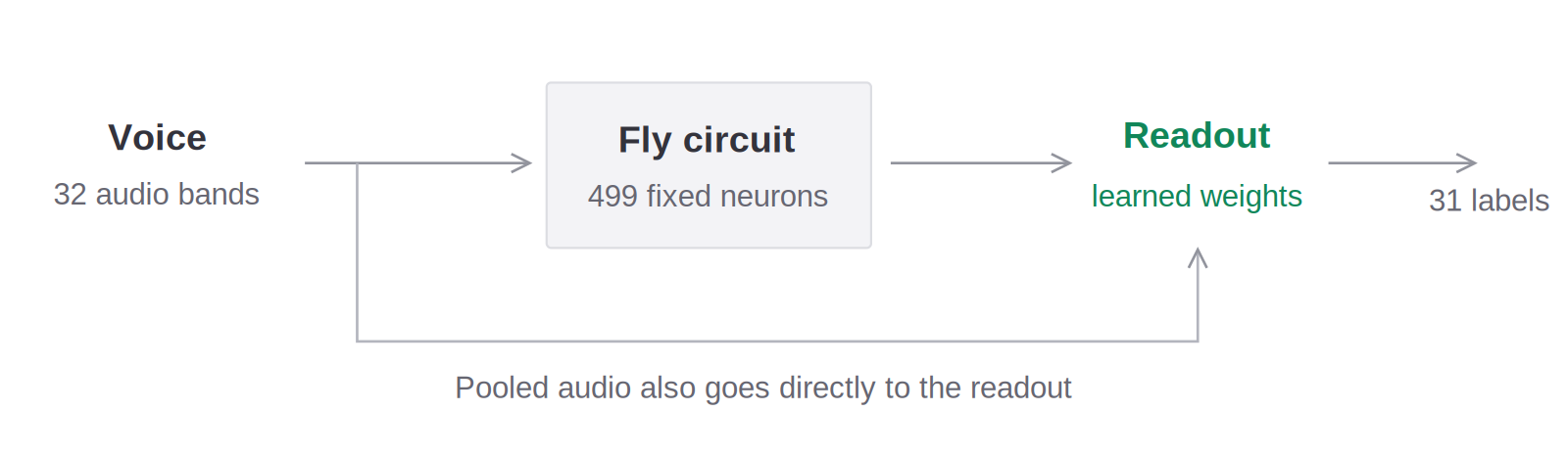
It's worth being precise about what's fixed and what's learned, because it's a much smaller footprint than "fly brain learns emotion" suggests. Audio is resampled to 8kHz, turned into 32 log-mel bands (25ms window, 10ms hop), normalized against training statistics, and clipped to ±5. That 32-dimensional signal enters the 499-neuron circuit through $W_{\text{in}}$ — a fixed random projection, not anything biological. So the only things standing between raw audio and a label are: a fixed random input matrix, a fixed (fly-shaped or not) recurrent matrix, and one trained linear layer.

That trained layer is small. Each recording's 499-unit activity gets summarized as four temporal means (early to late), concatenated into a 1,996-dimensional vector; a separate 128-dimensional pooled-audio feature vector is appended, giving 2,124 features per clip. A ridge regression maps that to 31 outputs — 15 emotion labels plus 16 speaking-style labels — and that's the entire trainable part of the model. The pooled-audio branch matters more than it sounds: it skips the circuit entirely, and the post says so itself — "some of what this model predicts can come straight from the voice without passing through the fly circuit." The whole thing, reservoir and readout together, is genuinely this small:

import numpy as np
 
def reservoir_states(W, W_in, U, alpha=0.15):
    """W: (499, 499) fixed weights, already rescaled to spectral radius 0.9.
    W_in: (499, 32) fixed random projection. U: (T, 32) log-mel frames.
    Nothing here is learned -- W and W_in never move."""
    x = np.zeros(W.shape[0])
    states = np.empty((len(U), W.shape[0]))
    for t, u in enumerate(U):
        x = (1 - alpha) * x + alpha * np.tanh(W @ x + W_in @ u)
        states[t] = x
    return states
 
def clip_features(states, audio_feats, n_bins=4):
    """4 temporal means of the 499 states, concatenated with 128 pooled
    audio features -> one 2,124-dim vector per clip."""
    chunks = np.array_split(states, n_bins, axis=0)
    means = np.concatenate([c.mean(axis=0) for c in chunks])
    return np.concatenate([means, audio_feats])
 
def fit_ridge(X, Y, lam=10.0):
    """X: (clips, 2124), Y: (clips, 31) soft multi-label targets.
    Closed-form ridge -- the only training step in the entire model."""
    Xb = np.hstack([X, np.ones((len(X), 1))])
    beta = np.linalg.solve(Xb.T @ Xb + lam * np.eye(Xb.shape[1]), Xb.T @ Y)
    return beta[:-1], beta[-1]

That's the whole trainable surface: one ridge solve. Everything upstream of fit_ridge runs once and never updates. If you wanted a one-line argument that this is reservoir computing and not a connectome finding, this is it — the "biological" part of the model has exactly the same job as a fixed random matrix would, and the code doesn't care which one it is.

The control that undoes the headline

Training used 16,995 clips, validated on 2,239, tested on 2,022 — drawn from 21,256 distinct waveforms and 21,600 retained ratings across CREMA-D and CSTR VCTK 0.92, with speaker and corpus groups kept entirely within one split. Most clips carry one listener rating; where a recording has several, they become soft targets, and a label counts as positive if at least half the available ratings picked it.

The headline metric is mean average precision (mAP), not accuracy, and that distinction matters here. With 31 labels and most of them rare in any given clip, a model that just predicts "not this label" for everything would score high on raw accuracy while being useless — mAP instead asks, for each label, how well the model ranks the clips that actually have it above the clips that don't, then averages that ranking quality across all 31 labels equally regardless of how common each one is. 16.84% mAP is not "16.84% accurate"; it's a modest but real ability to rank positives above negatives, well above chance, on a genuinely hard 31-way soft-label problem.

Against that metric, the authors ran four variants and compared them with 500 paired bootstrap resamples over the 45 held-out speaker/corpus groups, averaging three prespecified seeds per reservoir architecture (the audio-only baseline has no seeds — it's deterministic):

Four things are worth separating out:

• Fly vs. scrambled wiring (16.84% vs. 16.88%): difference −0.04pp, 95% CI [−0.16, +0.07] — squarely contains zero. The specific pattern of who-connects-to-whom, inherited from a real fly, buys nothing measurable over a random pattern with the same degree sequence and weights.
• Fly vs. audio-only (16.84% vs. 16.28%): difference +0.56pp, CI [−0.24, +1.37] — also contains zero. Even "having a reservoir at all, fly-shaped" over "no reservoir, just the audio features" isn't clearly resolved on this test set.
• Fly vs. no recurrent connections (16.84% vs. 16.61%, i.e. the same units and inputs with every neuron-to-neuron edge zeroed out): difference +0.23pp, CI [+0.04, +0.35] — this one doesn't cross zero. Having some recurrence, any recurrence, reliably beats having none, by a small but real margin.
• Constant scores (always predict the base rate): 9.71% mAP. This is the floor that says the other four numbers are measuring something rather than nothing.

Put together, that's a remarkably clean picture: recurrence-in-general helps a little; which particular recurrent structure you use doesn't help at all. That is precisely the standard reservoir-computing finding — a fixed nonlinear dynamical system followed by a linear readout beats a linear baseline, and the system's statistics (spectral radius, sparsity, weight scale) matter far more than its identity. It is not, on this evidence, a connectome finding.

The lesion experiment doesn't save the fly

The post runs one more experiment, and it's the most instructive thing on the page — because at first glance it looks like it contradicts everything above. Hold the trained readout fixed, then silence the 50 neurons with the largest readout weights (removing their incoming, outgoing, and input connections, no retraining). On one angry-labeled recording, the anger score drops from +0.29 to −0.43. Across the test set, mAP for that fitted model drops from 16.91% to 10.83% — a big fall, and a properly disclosed inconsistency: the paper notes the single-model 16.91% "differs from the 16.84% three-seed mean" because it's one specific fit, not the averaged headline number.

It's tempting to read that as "so the wiring does matter after all — look how much silencing 50 real neurons hurts." It doesn't say that, and the authors say why, cleanly:

"There is no contradiction between this result and the scrambled control. A readout learns to use the features its circuit produces. Remove part of that circuit after training and the features change under it. Give a different circuit its own training run and its readout can learn to use different features just as well."

This is the general shape of a mistake that shows up constantly in interpretability work: fit a readout to whatever a fixed system happens to produce, then break part of that system without refitting, and of course performance drops — you've pulled the rug out from under a readout that has no way to adapt. That's true whether the system is a fly connectome, a scrambled connectome, or a transformer's residual stream. It tells you the readout depended on those units for this particular fit. It does not tell you those units are special, biologically important, or a better starting point than any other 50 units would have been in a circuit trained to use them. The scrambled network, given its own training run, would build its own load-bearing 50 neurons — just different ones — and lesioning those would hurt just as much. Sensitivity-after-training and importance-of-the-substrate are different claims, and only the first one is what a lesion experiment like this actually measures.

What this does and doesn't say about emotion

One more thing worth being straight about, because the site's whole framing leans on it: emotion recognition from speech is a contested task, and the authors don't pretend otherwise. The labels here are listener judgments, not ground truth — "display labels come from listener judgments and can differ from the emotion an actor was asked to perform" — and a meaningful share of the training data (CREMA-D) is acted speech, professional performers reading lines to a target emotion, not people spontaneously feeling things. The six illustrative recordings shown in the post's activity visualizations are held-out positive examples selected for the demo, not a claim that any neuron encodes an emotion: "calling the indigo cells 'sadness neurons' would turn a color choice into a finding." And the authors are explicit about the ceiling on the whole exercise: "this experiment says nothing about whether a living fly understands human feelings." It's a listener-perception classifier with an unusually shaped set of fixed weights, tested against what humans said they heard.

Give the authors their due

None of this is a takedown. It's the opposite. The interesting scientific move here isn't "fly brain recognizes emotion" — it's that a team built a striking, clickable result and then ran and published, prominently, in the main text, the control that shows their own headline doesn't hold up. That's rarer than it should be, and it's the reason this piece was worth writing at all: not because the fly's connectome does something special, but because the honest version of the story — a fixed random-ish recurrent network plus a small linear readout, à la conn2res, wearing a fly costume — is still a real, useful reservoir-computing result, correctly caveated, with its own null result reported right alongside the headline number. That's what good science looks like when nobody's trying to sell you anything, and it's worth more than the version of this post that stopped at the 3D neuron renderer.