2026-07-21 · 8 min · reinforcement-learning · long-context
Why read this
Solidtop 85%How LongStraw fits 2M-token GRPO steps on eight H20s by capturing the prompt as resident state and replaying one response at a time, and what it does not claim.
- A new technique
- Open code or weights
- Explained from first principles
Training & RLNeeds datacenter GPUsResearch paper
How this was scored
- Is it new?
- 2 of 3: A real new idea, method or capability
- Can I trust it?
- 1 of 3: Spot-checks a few numbers
- Can I run it?
- 2 of 3: Open code or weights with real limits
- Will I understand it?
- 2 of 3: Mechanism from first principles with figures
- Can I act on it?
- 1 of 3: General advice
- Will it last?
- 1 of 3: Relevant for months
- Does it affect many?
- 1 of 3: A specialist community
- Only here?
- 1 of 3: Some original analysis
Score 48 of 100, ranked 478 of 577 rated articles. Each question is answered 0–3 by hand, and a 3 is rare. How articles are scored
There's a widening gap in how long a context a model can use versus how long a context you can train it on with RL. Inference servers now run million-token windows; RL post-training, as publicly described, mostly sits at 256K tokens or below and leans on length generalization at deployment. That gap matters most for agents, whose observations, tool outputs, retrieved documents, and past decisions pile up into the history that conditions the next action. LongStraw (MindLab and Fudan) sets out to close it — and it is unusually disciplined about framing the result as a systems feasibility claim, not an accuracy one.
Why GRPO is the hard case
Inference has an easy memory story: prefill the prompt, keep the state you need to decode, throw the forward graph away. GRPO can't. It samples G responses for one prompt and updates the policy from their relative rewards — so old-policy scoring, reference scoring, and every policy response all depend on the same long history, and policy learning must also retain or reconstruct what backward needs. Quadratic attention plus long-lived backward state make GPU memory the wall. The paper's framing: the practical limit is state lifetime, replay, and distributed ownership — not the attention kernel alone.
The move: change the graph boundary
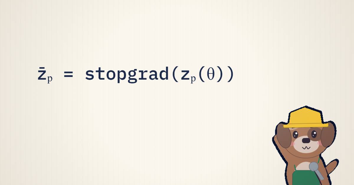
LongStraw's core data structure is resident state: evaluate the shared prompt with no autograd and keep only the minimal, model-native state later tokens need — recurrent state, KV pages, latent pages — not the full prompt activation graph. Formally it stores z̄ₚ = stopgrad(zₚ(θ)). Its core algorithm is response replay: restore that boundary, score the old and reference branches graph-free, rebuild one policy response under autograd, backpropagate, and pop back to the boundary.
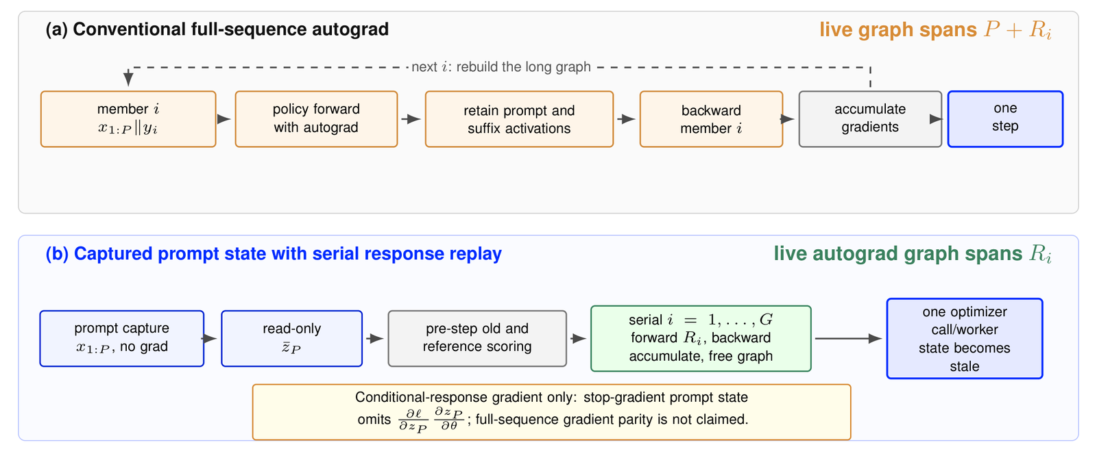
That last point is the honest heart of it. A full-sequence gradient has two terms — the direct response gradient and the prompt-side term that flows back through zₚ(θ). LongStraw keeps the first and drops the second. In the paper's own words, printed right on the figure: "conditional-response gradient only … full-sequence gradient parity is not claimed." The measured objective is response-only execution.
Serial replay makes G a schedule, not a memory multiplier
Because responses are replayed one at a time, the live autograd graph is bounded by a single response — so the group size G becomes a scheduling/time dimension instead of a memory multiplier. This is the lever that makes million-token steps fit. Drag G and watch the measured peak barely move:
On eight H20 GPUs, Qwen3.6-27B completes an exact-attention response-only GRPO step at 2,097,152 positions for both G=2 and G=8 — and going from G=2 to G=8 adds only 0.208 GB of peak allocated memory per rank (97.503 → 97.711 GB). Holding all G response graphs, by contrast, would scale activation memory with G and overrun the budget. That's the trade the design makes: G costs wall-clock (271 s per member), not memory.
Two incompatible architectures, same transaction
The design is instantiated for two structurally different models, which is most of the engineering:
- Qwen3.6-27B (8× H20, CP8) — 48 Gated-DeltaNet layers + 16 full-attention layers, dense FFNs. It keeps compact recurrent state for GDN and right-sized CP8-sharded KV pages for full attention, composes rank-local softmax statistics into the exact global attention output, replays response blocks in reverse, and allocates K/V gradient pages only when a response backward touches them. NF4 QLoRA, 116.7M trainable parameters.
- GLM-5.2 (32× H20, CP32/EP32) — 78 MLA/DSA attention layers (21 index + 57 IndexShare) and a 3-dense/75-MoE feed-forward stack routing each token to 8 of 256 experts (+1 shared). It holds CPU-resident MLA latent pages and DSA index-key pages, reconstructs the sparse selection across context-parallel owners, and replays the real Megatron router, EP32 all-to-all, and expert compute under whole-layer checkpointing. (This is the same GLM 5.2 whose IndexShare makes a million-token context cheap.)
Qwen solves preserve and replay dense/recurrent history; GLM extends it to dynamic sparse selection, routed experts, and cross-rank communication.
The numbers, and the ceiling
The headline is how far the training context moves — from the usual quarter-million to millions of positions on fixed hardware:
At 4,456,448 positions, one captured prefix supports eight consecutive G=8 optimizer cycles — 64 response replays — at 83.894 GB per rank, comfortably under the H20's 150.755 GB. On 32 H20 GPUs, GLM completes a deterministic 2M execution across all 78 layers with two full backward passes. The memory plot shows how the operating points sit against the ceiling:
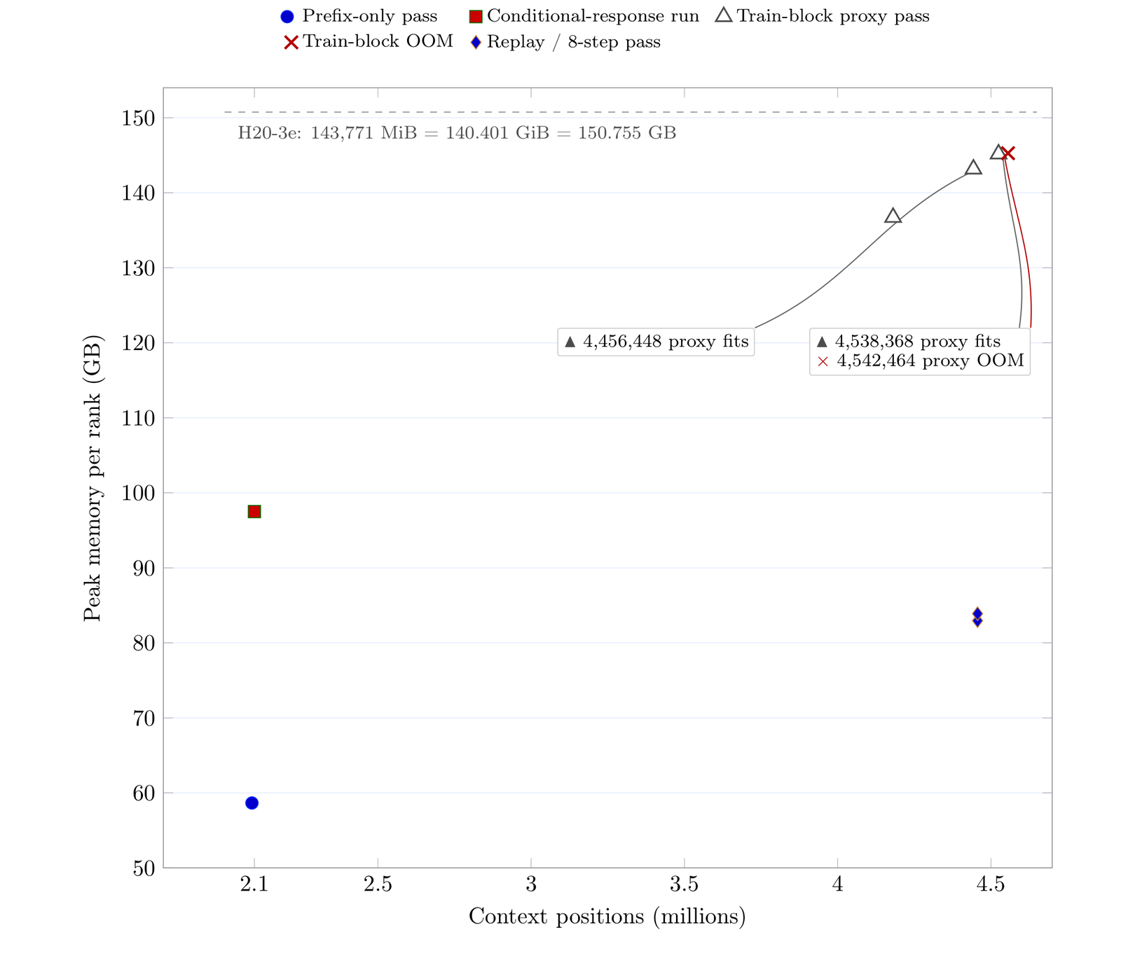
Note what the plot says and doesn't: 2M is "an achieved operating point rather than a measured capacity ceiling." They ran it; they don't claim it's the max.
The refresh knob
Capturing a million-token prompt is the dominant cost, so LongStraw reuses one capture across several optimizer steps. But each update moves the parameters, and the cached prompt state goes stale. A 1M fresh-prefix oracle measures exactly how stale — and turns "how long can I reuse a prefix" into a number:
Reuse is nearly free for a step or two (loss drifts ~0.04–0.12%) and clearly not by step four. So the refresh interval becomes a measured control, not an assumption.
The fine print (which is the point)
This is where LongStraw earns its credibility. It defines four levels of validation and states plainly where each path lands:
Spelling that out is not a weakness of the paper — it's the substance. A lesser report would have shown a 2M run and let you assume it means a better model. LongStraw shows a 2M run and tells you exactly which narrow, well-defined thing completed.
The take
The useful reframing here is that long-context RL is a state-lifetime and ownership problem, not an attention-kernel problem. Once you treat the long prompt as detached resident state and replay responses serially, the memory transaction — not the kernel — is what sets how far you can train, and million-token steps fit on inventory you already have. It's a real feasibility milestone, and it sits next to the other systems-first takes on RL cost like frontier RL is cheaper than you think. What's left — and the paper is the first to say it — is closing the distance from "the step executes" to "the gradient is exact and the policy actually improves at 2M tokens." That's the next paper, honestly labeled.
Source: LongStraw: Long-Context RL Beyond 2M Tokens under a Fixed GPU Budget (Zhou et al., MindLab & Fudan University), July 2026. Figures are the paper's; the two interactives are mine, built on its measured numbers.