2026-10-31 · 15 min · retrieval · vector-search · on-device · benchmarks

Why read this
Essentialtop 10%Rebuilds the 97% from byte arithmetic, then builds LEANN and HNSW over 20,000 chunks: index 91% smaller, but 663 to 2,768 embedder calls and 25 to 92 s a query.
- Original, source-checked analysis
- Runs on a laptop CPU
- Interactive explanations
Developer tools & infraMITPractitioner teardown
How this was scored
- Is it new?
- 2 of 3: A real new idea, method or capability
- Can I trust it?
- 3 of 3: Reproduces the headline result, or shows from primary files it is wrong
- Can I run it?
- 3 of 3: Open, permissive, runs on reader hardware with instructions
- Will I understand it?
- 3 of 3: Mechanism carried by interactives built from real code or data
- Can I act on it?
- 3 of 3: A decision guide a practitioner can follow today
- Will it last?
- 2 of 3: A reference for a year or more
- Does it affect many?
- 2 of 3: A widely used model, tool or lab release
- Only here?
- 3 of 3: The only place this analysis exists
Score 92 of 100, ranked 1 of 666 rated articles. Each question is answered 0–3 by hand, and a 3 is rare. How articles are scored
A post making the rounds says LEANN, an open-source project, "compresses 60 million text chunks from 201 GB to just 6 GB, with no accuracy loss in its tests, running locally." That is a 97% cut to a vector database, which is a lot to believe from one sentence. A vector index that stays accurate usually keeps the vectors, and the vectors are most of the bytes.
So I did three things. I read the paper and the repository. I did the byte arithmetic until the 201 and the 6 either came out or didn't. And I built a LEANN index and a plain FAISS HNSW index over the same 20,000 text chunks, on two CPU threads, and measured size, recall and what a query costs. Each claim below is tagged measured (a number from my runs), reported (the paper or README says so, I did not reproduce it) or reasoned (I derived it from numbers I did have).
The short version. The 97% is real in structure: LEANN does not store the vectors. On my corpus the index file shrank by 91%, and the arithmetic says it would be about 95% at the 768-dimensional size the post is about. The cost is that every graph node a query visits is now a forward pass through an embedding model. On my machine that was 663 to 2,768 passes per query, 25 to 92 seconds. The paper gets to a couple of seconds with a GPU and two ideas the released code does not use by default. Both halves are worth knowing before you put it near a laptop.
- license
- MIT
- branch
- main
- tests
- 73 files
- source
- 2.1 MB
- commit date
- 2026-10-28
by size of tracked source at this commit, file counts in brackets; docs, data and vendored trees excluded
local clone, 2026-10-31 at 07796bd — branch, commit, commitDate, fileCount, hasTests, languages, license, licenseFile, shallow, testFileCount
shallow clone: counts describe the pinned tree, not the history
Where the numbers come from
The post's figures are in the repository's README: a table with "Wiki (60M)" at 201 GB for "a traditional vector database (e.g., FAISS)" and 6 GB for LEANN, a 97% saving. The paper does not contain those two numbers. It contains these, for the same 60-million-passage Wikipedia datastore (RPJ-Wiki, 76 GB of raw text, 256-token chunks embedded by Contriever into 768-dimensional vectors):
| HNSW | LEANN | |
|---|---|---|
| Vectors | 173 GB | 2 GB (PQ codes) |
| Index metadata (the graph) | 15 GB | 2 GB |
| Total | 188 GB | 4 GB |
Reported, from the paper's Table 1 and Figure 3. One minus 4 over 188 is 97.9%, which the paper rounds to "over 97%". One minus 6 over 201 is 97.0%. So the README's headline and the paper's agree on the percentage and disagree on both inputs. I can't reconstruct why from either source, which I note and move on from; I come back to the 201 below, where it does come out of the arithmetic.
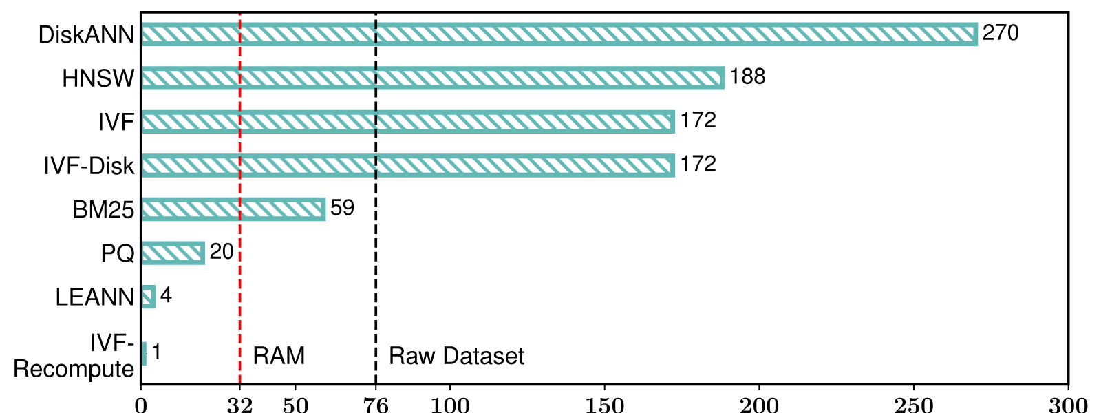
Notice what the bars leave out. The 76 GB of raw text is in none of them, because every method has to keep the text it returns, and LEANN also needs it as the input to every recompute. The paper's own phrase is "below 5% of the original data", and 4 over 76 is 5.3%.
What an HNSW index stores
HNSW is a graph. Every chunk is a node. Each node holds a list of the ids of nearby nodes, and a
query walks the graph: start at an entry node, look at its neighbours, move to whichever is closest
to the query, keep a queue of the best efSearch candidates seen so far, stop when the queue has
nothing left to improve. It never scans the corpus. The reason it is fast is that it computes a
distance to only a few thousand vectors, not 60 million.
To compute a distance you need the vector. So the standard index stores two things per node:
- the vector,
dfloats of 4 bytes each; - the neighbour list. FAISS pads the bottom layer to
2Mids per node whether they are used or not, so withM = 32that is 64 ids of 4 bytes, 256 bytes.
The arithmetic for the 60M corpus. Reasoned:
- Vectors: 60,000,000 x 768 x 4 = 184.3 GB, or 171.7 GiB. The paper says about 173 GB. Within a percent, if you read it in GiB.
- Graph: 60,000,000 x 256 = 15.4 GB. The paper says 15 GB.
- Sum: 199.7 GB. The README says 201 GB.
So the 201 is, to within 0.6%, "fp32 vectors plus a padded HNSW graph". That is the right baseline. Nothing about it is a strawman. It is also the entire premise: the vector is 92% of that index. Remove it and a 90%-ish saving falls out before any cleverness.
The widget does the arithmetic above for three corpus sizes. Leave the sliders at the paper's values (average degree 9, a 33-byte PQ code) and you get the paper's 4 GB at 60M. Set PQ to 0 and the degree to 40 and you get what I measured the released code to build, further down.
The trick: recompute what you visit
LEANN's first idea follows from the arithmetic. A graph search visits a few thousand nodes out of millions. If you do not store the vectors, you can compute only those few thousand from the text, at query time, with the same embedding model that built the index. The graph tells you where to look; the embedder supplies the vector when you get there.
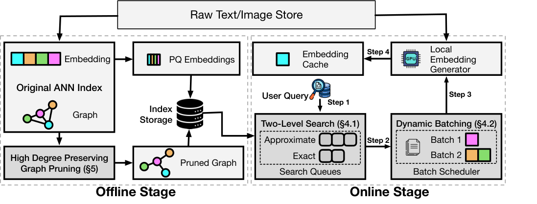
The paper adds four things on top of that, all reported:
- High-degree preserving pruning. The graph is still 15 GB at 60M. Most nodes are rarely visited; a few hubs with many edges are visited constantly. So cut the edges of low-degree nodes and keep the hubs' edges. The paper keeps the top 2% of nodes by degree at full degree and holds the rest to a smaller one, and gets an average degree of 9 from 18 with search quality close to the unpruned graph.
- Two-level search. Keep a small PQ code per node (about 33 bytes against 3,072 for the fp32 vector). Use the cheap approximate distance to rank a node's neighbours, then recompute exact vectors only for the best few. This is what keeps recomputes down. Without it, every neighbour touched costs an embedder call.
- Dynamic batching. A GPU is wasteful on 5 texts. Collect candidates across several steps of the search until there are about 64, embed them together. It trades a slightly stale visit order for throughput.
- An optional embedding cache for hot nodes, if you have disk to spare.
The reported payoff is in the paper's Table 2: retrieval at 90% recall takes 2.48 s for LEANN on Natural Questions against 0.05 s for HNSW, on an RTX 4090, with generation at 20.86 s. That is 10.6% of the pipeline. The argument is that an LLM answer takes ten seconds anyway, so seconds of retrieval are cheap. It is a good argument if your retrieval is followed by a large model on a GPU. It is a different one if it is not.
What I ran
I did not have 76 GB of Wikipedia or a GPU, so I built the same experiment at 1/3,000th the size.
Corpus. 25 Project Gutenberg books (public domain), cut into 100-word chunks, shuffled with a
fixed seed, first 20,000 kept. Embedder. all-MiniLM-L6-v2, 384-dimensional, normalised, run
through LEANN's own compute_embeddings on 2 CPU threads: 787 seconds for the 20,000, about 39 ms
a chunk. Queries. The first 16 words of 100 held-out chunks from the same books. Not realistic
questions, but they have real neighbours. Ground truth. Exact inner-product search over the
stored vectors, top 10. Indexes. Both built with M = 32, efConstruction = 200:
faiss-cpu 1.15.1's IndexHNSWFlat, and leann-backend-hnsw 0.3.8 through LeannBuilder with
its defaults (is_recompute=True, is_compact=True). I ran the released package from PyPI, not a
build of the source, and the C++ fork it wraps is not something I could read (more on that below).
Size
Measured, bytes on disk:
| FAISS HNSW | LEANN | |
|---|---|---|
| Vectors | 30,720,000 | none |
| Graph | 5,442,530 | 3,234,570 |
| Index file | 36,162,530 | 3,234,570 |
| Passage text, offsets, ids | 12,513,786 | 12,513,786 |
| Everything you must keep | 48,676,316 | 15,749,022 |
The index file is 8.9% of the size, a 91.1% saving. That is the 97% claim's real number at this scale, and it is lower for a reason. 384-dimensional vectors are 1,536 bytes a chunk, half of 768-dimensional ones, so removing them saves less. Reasoned: with the same graph and 768-dimensional vectors the baseline is 66.9 MB and the saving is 95.2%. At 60M with the graph I measured, 161.7 bytes per node, the LEANN graph would be 9.7 GB against 199.7 GB, a 95.1% saving.
The last row is the one to remember if you are budgeting a laptop. LEANN's directory is 15.7 MB. Of that, the index is 3.2 MB and the text is 12.2 MB, almost four times as much. A baseline that also needs the text is 48.7 MB, so the whole-deployment saving is 67.6%, not 91%. The text has to stay: it is what you return, and it is what you re-embed.
Query cost
I ran LEANN on 15 queries at each of complexity 16, 32 and 64 and on 6 at 128, because they are
slow, and counted the texts the embedding server was asked to embed from its own log.
| efSearch | FAISS recall@10 (100 q) | FAISS distance computations | LEANN recall@10 | LEANN texts embedded | LEANN seconds per query |
|---|---|---|---|---|---|
| 16 | 0.802 | 664 | 0.847 | 663 | 25.3 |
| 32 | 0.903 | 1,044 | 0.947 | 1,045 | 39.1 |
| 64 | 0.963 | 1,728 | 0.973 | 1,757 | 64.1 |
| 128 | 0.991 | 2,867 | 0.983 | 2,768 | 91.8 |
Measured. Two things are in that table.
The recall is the same. The LEANN column is on 6 to 15 queries and so noisy (a miss or two moves a 15-query mean by 0.01 or more), and the two indexes are separate graph builds, so some wobble is expected. Nothing in it says recomputing hurts accuracy. The paper's own claim, that downstream QA accuracy matches HNSW once both are tuned to 90% recall, is reported, not something I tested.
The work is the same too, which is the point. LEANN embedded 663 texts per query where FAISS did 664 distance computations, 1,045 against 1,044, 1,757 against 1,728. Every distance computation became an embedder call. Nothing was saved by being clever at query time, and it should not have been: the released path does not use the second idea.
At 20,000 chunks a query at efSearch 16 embeds 3.3% of the corpus. At 60 million the visited set
grows far more slowly than the corpus, which is the whole reason graph search works, so the fraction
becomes tiny. Reasoned: the count per query is what matters, and it stayed in the hundreds to low
thousands.
The time
25 seconds a query at the lowest setting, 92 at the highest, on two CPU threads of a shared four-core box that was running other people's jobs at load 5, so read the absolute seconds as an upper bound. The ratio holds regardless: FAISS answered in 0.23 to 0.70 ms. That is about five orders of magnitude at equal recall.
The seconds track the texts at roughly 37 ms each (25.3 over 663, 91.8 over 2,768). That is the same
as the 39 ms a chunk I paid to embed the whole corpus in batches of 32. So on CPU, batching bought
nothing: the model is the cost. The server does batch inside a round (about 28 texts per round trip at
efSearch 16), and a GPU would eat that, but a laptop CPU does not get cheaper per text from it.
MiniLM-L6 has 22 million parameters. The paper's Contriever is BERT-base, about five times that. Reasoned: a like-for-like CPU run with the paper's embedder would be slower than mine.
What the shipped code does, against the paper
I read the Python in packages/leann-backend-hnsw and packages/leann-core at commit 07796bd (source version 0.3.9; the wheels I ran are 0.3.8).
Code reading, with each point something I checked, not inferred:
- The builder is
faiss.IndexHNSWFlat(dim, M, metric)withM = 32andefConstruction = 200defaults, then a conversion to compressed-sparse-row (convert_to_csr.py) that writes a "NULL" storage in place of the vectors. That is the "drop the vectors" step and the CSR layout the paper calls compact. - There is no degree-based pruning step in that Python, and no PQ table is built. The two-level
search's knob exists:
prune_ratiois passed through to the C++ search aspq_pruning_ratio. It defaults to 0.0 inLeannSearcher.search, in the CLI, and in theHNSWSearcher, and I ran with the default. I did not turn it on. A pruned index has no PQ codes to prune with, as far as the Python shows. - I found no hub-node cache in the Python. The only cache there is for query embeddings.
The graph's own size says the same thing. LEANN's index file is 3,234,570 bytes for 20,000 nodes,
161.7 bytes a node, about 40 neighbour ids. I read the degree distribution of the plain FAISS graph
with the same parameters: 658,173 edges, a mean of 32.9 per node, a maximum of 64 (the 2M cap), and
the top 2% of nodes by degree own 3.9% of the edges, so no hub structure shows up. Those edges at 4
bytes plus the offsets are 2.79 MB, close to the 3.23 MB file. Reasoned, and it is not proof: it
fits a CSR-compacted, unpruned HNSW graph, and the paper's pruned graph would be about 33 bytes a node
(2 GB over 60M), five times smaller than mine. The pruning and PQ code may live in the C++ fork the
wheel wraps, which I could not read: the submodule is not in the checkout and I did not build it.
So when the README says "97% less storage without accuracy loss", the part I could confirm is the
bigger half: the vectors are gone. The graph squeeze and the speed-ups that make it usable are in
the paper, and I could not find them in what runs by default. The repo's benchmarks/ and the
README's "Reproduce Our Results" would be where to look; I did not run them (they pull a large
evaluation set).
When this is the right tool
Reasoned from the numbers above, not tested in an application.
It fits when disk is the scarce thing and queries are rare. An email archive, a browser history, a notes folder: the README's examples of 780,000 email chunks in 79 MB or 38,000 browser entries in 6.4 MB are reported and I did not check them, but they are the right shape. You search a few times an hour, you can wait, and the alternative is an index several times the size of the thing it indexes.
It does not fit when queries come in a stream, when there is no GPU and the embedder is more than a small model, or when the vectors would have fit in RAM anyway. At 25 seconds a query you cannot interactively search, and a handful of concurrent users would saturate the embedder.
And if what you want is a smaller index and not an absent one, there are cheaper first steps that keep a vector in the index:
- Truncate or quantise the vector. Product quantisation to 33 bytes, the paper's PQ column, takes the vectors from 173 GB to 2 GB by itself. The paper's complaint is that at that ratio, plain PQ search loses accuracy ("fails to reach 90% recall", as reported). Use PQ as a shortlist and re-rank from text, which is what two-level search does.
- Memory-map the stored vectors and let the disk page them. You pay in latency the way LEANN does but you keep the vectors on disk, which costs little compared with an embedder forward pass per node.
What I did not run
- The paper's setting: 60 million chunks, Contriever, an RTX 4090. Every number from there is reported.
- The two-level search with PQ, dynamic batching, and the hub cache. If they live in the C++ fork I could not read it, so I can't say what they would have saved on my corpus.
- Any downstream QA, so "no accuracy loss" is tested only as recall@10 against exact search.
- More than 15 queries per setting for LEANN, so its recall column has wide error bars.
- The README's email, chat and browser numbers.
If you run this yourself, the setup is pip install leann-core leann-backend-hnsw, build with
LeannBuilder(backend_name="hnsw", is_recompute=True, is_compact=True), and count the texts by
setting LEANN_LOG_LEVEL=INFO and summing the embedding server's Computed embeddings for N texts
lines.